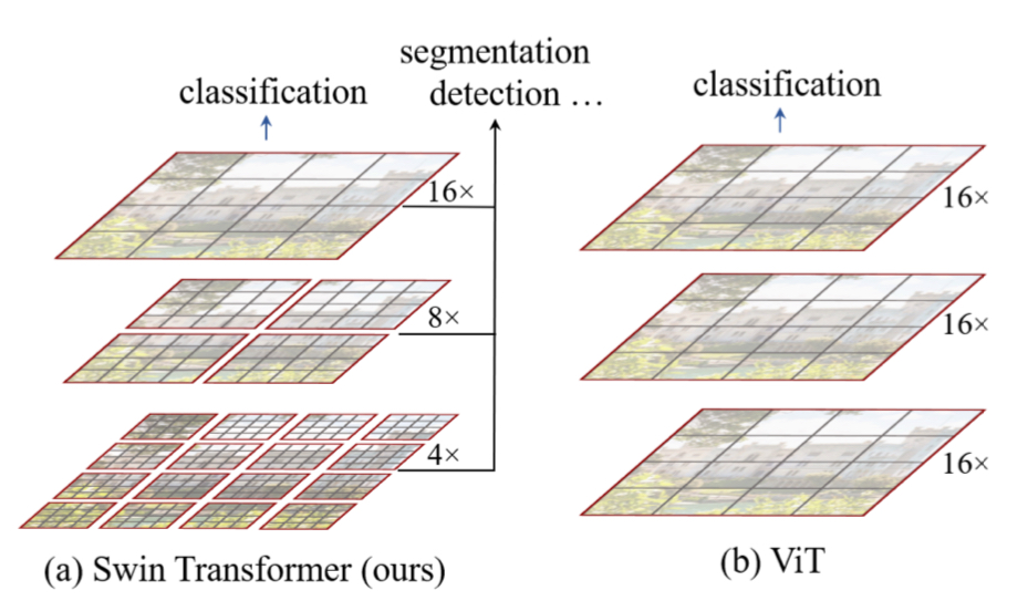
Liu, Ze, et al. "Swin transformer: Hierarchical vision transformer using shifted windows." Proceedings of the IEEE/CVF international conference on computer vision. 2021.
Introduction
Transformers have shown its strong performance in natural language processing, and have dominated the area to serve as the de facto standard backbone architecture. However, it was not until the advent of Vision Transformer (Korean) that pure transformer-based models without dependence to the traditional CNNs have been prevailing over the field of computer vision. The ability of attention module to capture global dependences with relatively less parameters turned out to be highly effective for image recognition tasks.
Despite the high performance, ViTs had fundamental problem in its scalability. Due to the behavior of self-attention, ViT is bound to have quadratic time complexity to the image size, i. e. $\Omega((hw)^2)$. This sometime is incompatible to the inherent nature of vision tasks having highly varied size of input. ViTs are also barely applicable to various tasks other than classification.
Researchers of Microsoft came up with Swin(Shifted Windows) Transformer to alleviate these problems. Exploiting its hierarchical architecture and shifted windows approach, the model captures the long-distance dependences in the image without directly calculating the global self-attention, which necessarily incurs quadratic time complexity. As a result, the model achieved the state-of-the-art performance while maintaining linear time complexity.
This article delves into the problems of the established Vision Transformer and how the authors leveraged the newly devised architecture to surmount these issues. Additionally, we explore Video Swin Transformer which was later suggested by the authors as an application of the Swin Transformer adapted for video processing.
The pioneering work of Vision Transformer (ViT) have achieved an impressive performance in computer vision tasks with the architecture purely based on the attention mechanism. However, there arises a couple of problems due to the difference between the two domains, NLP and vision.
-
Varied scale of semantic elements
Visual elements can vary a lot in its size. For example, a visual element depicting a dog may occupy virtually the entire image, or may be as small as a chunk of few pixels. This contrasts with natural language tasks where only one or a few tokens constitutes the fundamental element that bears meaning.
-
Higher resolution of pixels
Pixels are the basic building blocks of images, and thus are on par with tokens of passages. Unlike sentences in NLP tasks, images are composed of a vast number of pixels. This is especially problematic for tasks that require pixel-wise prediction such as semantic segmentation, since the computational demand quadratically increases with the input size.
The authors cope with each of the problems by coming up with a hierarchical architecture which employs shifted windows: Swin Transformer.
- Varied scale of semantic elements: Swin transformer starts off with the embedding of small-sized patches, and merges them hierarchically to model the dependences in larger scale. Thus, it can process visual elements in varied scales.
- Higher resolution of pixels: By employing the hierarchical architecture, the model achieved linear time complexity. Thus, the model is compatible with larger size images and embraces extended range of tasks, including those that require pixel-scale predictions.
Method
Let’s take a deeper dive into the architecture introduced in Swin Transformer. As previously mentioned, the key features of the model can be summarized in two: (1) hierarchical merging of feature patches and (2) alternating shifted windows where local self-attention is calculated.

Hierarchical Patch Merging
The process of hierarchically building the feature map is the biggest contribution made in this paper. As opposed to ViT, which computes the self-attention globally in all layers, Swin Transformer starts from calculating the self-attention within a small windows.

Given the input image, the model partitions the original input image into patches of size $4\times4$, yielding total of $\frac{H}{4}\times \frac{W}{4}$ patches. This yields a collection of $4\times4\times3=48$-dimensional vectors, where 3 comes from the color dimension (RGB). The vectors are mapped with the linear embedding matrix to be projected to the embedding space (with dimension $C$), reshaping the data into $\frac{H}{4}\times \frac{W}{4}\times C$. These embedding vectors perform an identical role with that in NLP transformers. Up to this point, the data goes through the same process as in ViT.
After that, Swin Transformer partitions the image patches with a grid. This is where the self-attention is calculated. Thus, no calculation is performed between the image tokens that belong to separate cells in the grid, saving the computational budget greatly. This contrasts to the existing ViT, which calculates the self-attention between all possible pairs of patches. The matrix shape still remains $\frac{H}{4}\times\frac{W}{4}\times C$ (Stage 1).
This process of per-window self-attention is held repeatedly, but with a different grid size. This is where the idea of patch merging comes into the play. The following Swin Transformer blocks are preceded by the patch merging layer(see panel (a) in the figure above), which concatenates the neighboring $2\times2$ patches and applies a linear layer onto $2C$-dimension. Considering that the initial, four patches combined is $4C$-dimensional, this can be seen as 2x downsampling in resolution. Undergoing this process followed by two more swin transformer blocks, the matrix is further reduced into shape $\frac{H}{8}\times\frac{W}{8}\times 2C$ (Stage 2). The remaining stages 3 and 4 are held in the same way, resulting in the final matrix in the shape $\frac{H}{32}\times \frac{W}{32}\times 8C$.
Shifted Window based Self-attention
Then how is each Swin Transformer block constructed? The panel (b) in the figure above depicts the architecture of two consecutive Swin Transformer blocks. Those who are already familiar with ViT would realize that the diagram is exactly the same with it, except the self-attention replaced with W-MSA and SW-MSA, each of which representing regularly windowed multi-head self-attention and shift-windowed multi-head self-attention.
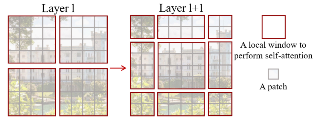
Here, the window being shifted means that the partitioning of the windows where the self-attention is calculated is displaced by half its size, in both directions(as in the figure above). This is to better model the relationship between the adjacent windows. If all the partitions were held in the same way, the model would compute the self-attention only within the same windows. By placing normal and shifted partitioning alternatively, the model introduces more connection between the adjacent windows, and thereby have a better understanding of the image.
This reduces the time complexity of Multi-head Self-attention of $M\times M$ patches with size $h\times w$ as follows:
- Original MSA: $4hwC^2 + 2(hw)^2C$
- Windowed MSA(W-MSA): $4hwC^2 + 2M^2hwC$
Thus, the windowing approach reduces the time complexity from quadratic to linear to the patch number $hw$, and thus more scalable and affordable to large images.
Two Configurations for Shifting
There are two ways in performing the window shift. One way is to partition the image as described above. Assuming an $8\times 8$ feature map, this yields $3\times 3=9$ windows (although the sizes differ) as in the figure above. Compared to the preceding regularly windowed block (which uses $2\times2=4$ windows), this incurs considerably more compute demand.

An alternative way to this is to introduce cyclic shift. As depicted in the figure, this approach concatenates the sub-windows on the edges to complete full-sized windows, where the computation of self-attention is performed. This reduces the number of windows into $2\times2=4$, which is same as regularly shifted blocks, and therefore prevents the additional computation due to shifting. However, on the other hand, the model begins to capture the dependences between irrelevant patches on the edges.
Relative Position Bias
Due to its permutation-invariant property, transformers require positional encoding to supply information about the token location. Unlike the original ViT architecture, which uses absolute positional encoding, Swin Transformer include relative position bias $B\in\mathbb{R}^{M^2\times M^2}$during the computation of self-attention:
$$\text{Attention}(Q, K, V) = \text{softmax}(QK^T/\sqrt{d}+B)V$$
where $Q, K, V\in\mathbb{R}^{M^2\times d}$ are the query, key, and value matrices with $d$ being the embedding dimension. Here, $B$ is composed up to add a different value based on the relative displacement between a query and a key patch. That is, given that a key patch $k$ has the relative position $(i, j)\in [-M+1, M-1]^2$ with respect to a query patch $q$, the bias added to the scaled dot product $\frac{q\cdot k}{\sqrt{d}}$ is retrieved from the element $\hat{B}_{ij}$ of the bias matrix $\hat{B}^{(2M-1)\times(2M-1)}$.
Experiments
The authors evaluated the model on three different datasets:
- ImageNet-1K image classification
- COCO object detection
- ADE20K semantic segmentation
ImageNet-1K Image Classification
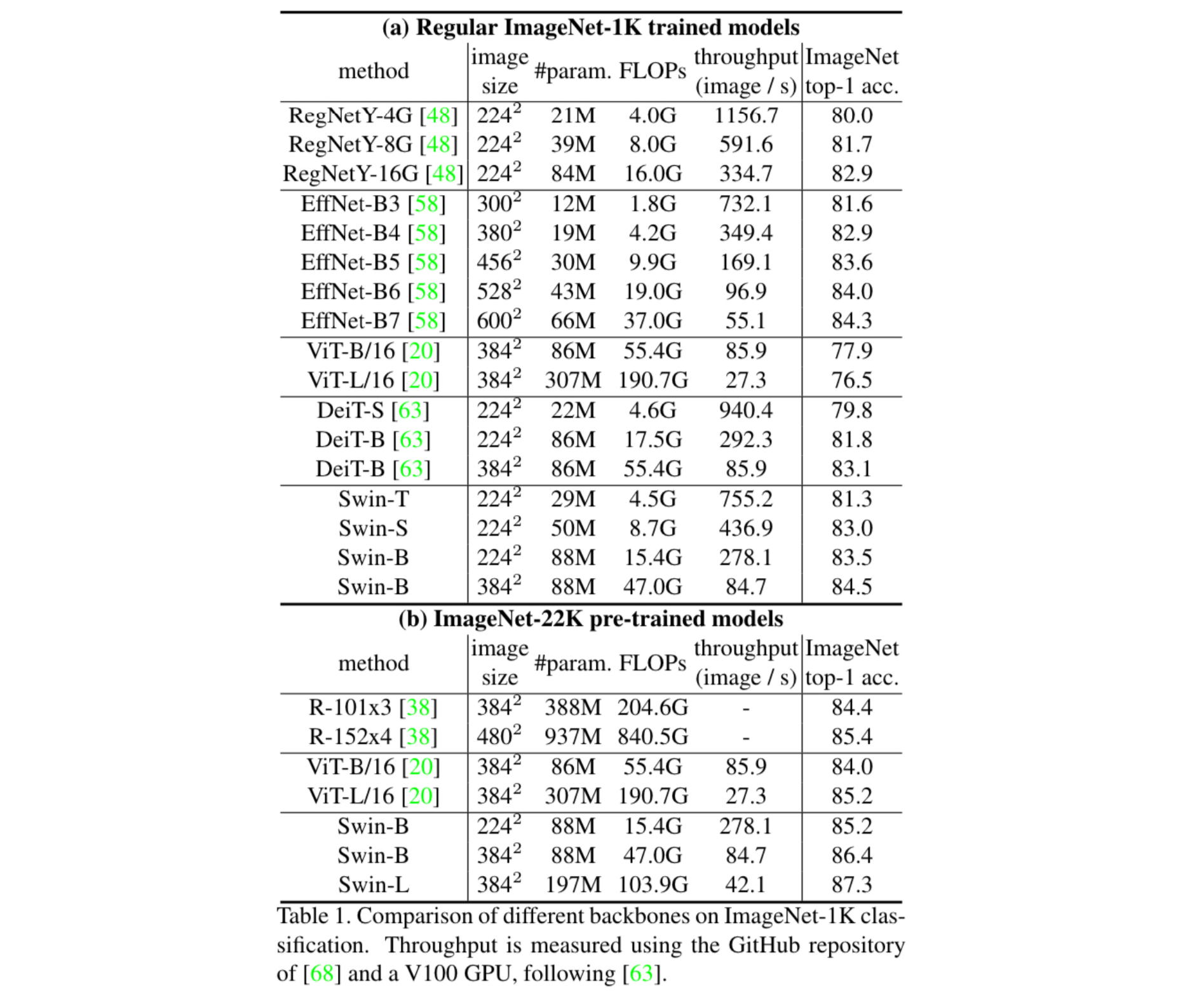
The authors trained Swin Transformer along with other models for comparison. They employed two different settings: (1) direct training on the ImageNet-1K, and (2) pre-training on ImageNet-22K, followed by fine-tuning on ImageNet-1K. In either cases, Swin Transformer attained a performance significantly surpassing the existing state-of-the-art architecture, DeiT.
COCO Object Detection
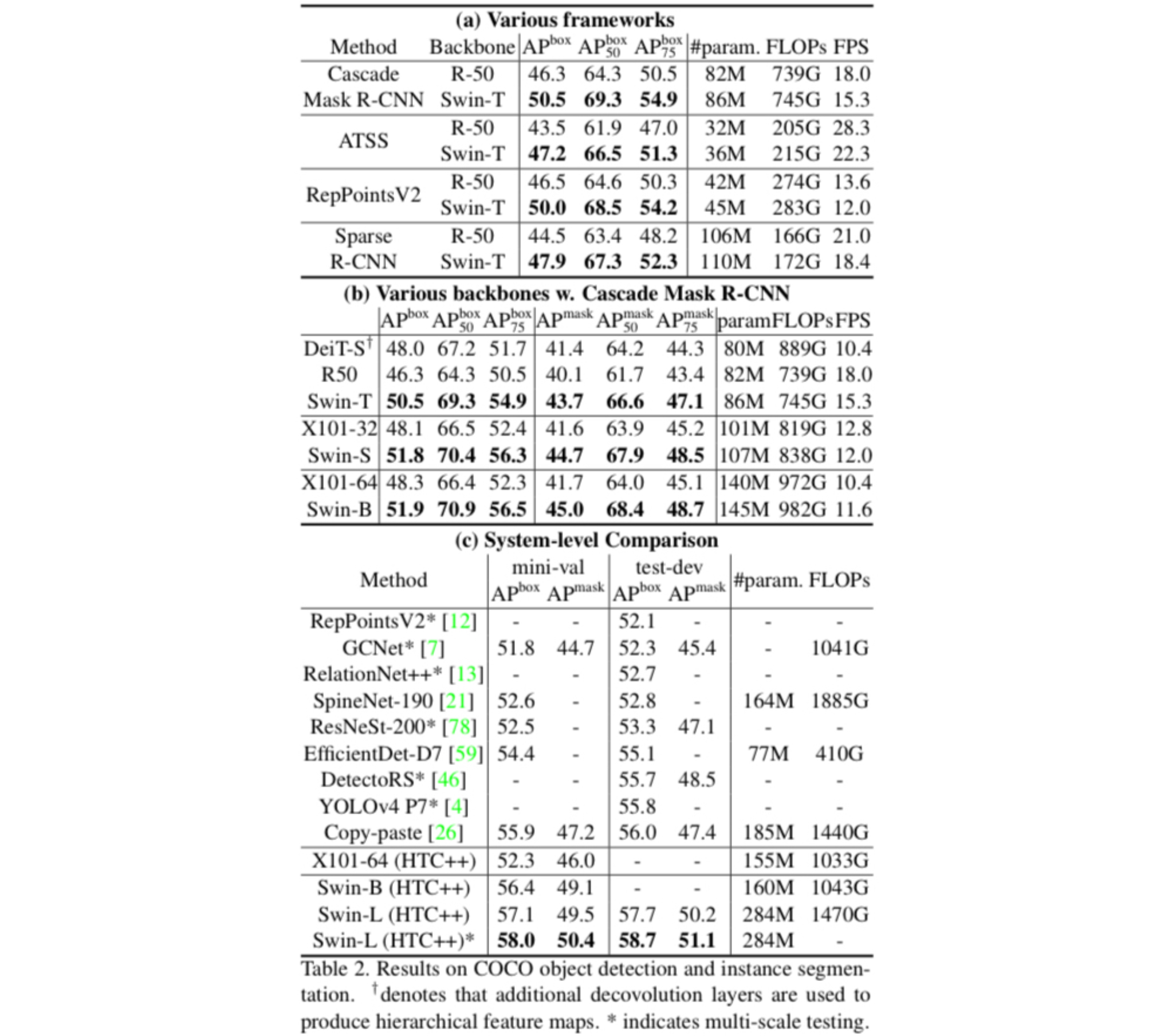
The authors assessed the performance of Swin Transformer on COCO object detection. Here, three different methods were used for evaluation.
- Firstly, the authors implemented four different frameworks: Cascade Mask R-CNN, ATSS, RepPointsV2, and Sparse R-CNN, with its backbone replaced with ResNet-50 and Swin Transformer-T(tiny). The authors observed the performance difference due to the underlying backbone. Swin Transformer outperformed ResNet50 in every combination of models and metrics.
- Secondly, more varied set of backbone architectures were compared with the framework fixed to cascade mask R-CNN. The employed architectures included DeiT, ResNet, and ResNeXTs, which were sorted according to its parameter size. In all three ranges of parameters, Swin transformer outperformed the other architectures.
- Lastly, A system-level comparison was conducted. The authors have employed HTC(Hybrid Task Cascade)and improved to build the model which they refer to as HTC++. The HTC++ employing Swin Transformer-L(large) achieved the new state-of-the-art performance.
ADE20K Semantic Segmentation
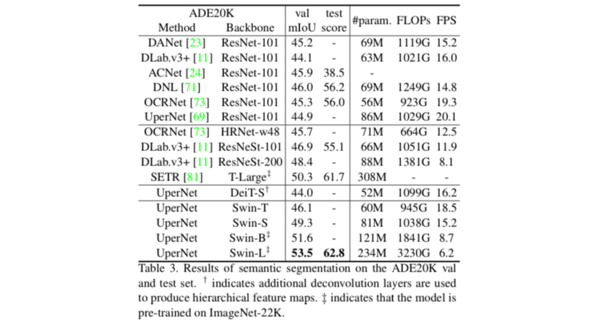
Finally, the authors evaluated the performance of Swin Transformer on semantic segmentation task. As demonstrated in the table above, architectures involving Swin Transformer surpassed the other models with comparable compute demands.
In their paper published a year later, the authors straightforwardly extended the architecture of the Swin Transformer to be applicable to the video domain, calling it the Video Swin Transformer. Considering video data as a $T\times W\times H\times 3$ matrix ($T$: number of frames), the authors modified details in the model while preserving the overall architecture.
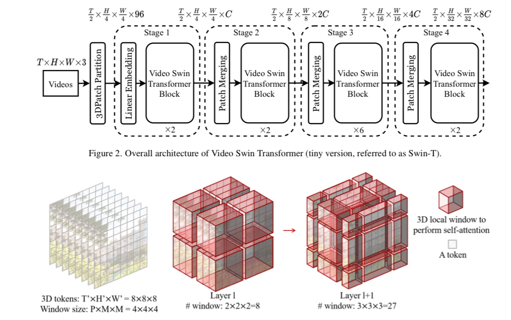
- The initial partitioning splits the data into 3D tokens of size $2\times4\times4\times 3$. Therefore, a total of $\frac{T}{2}\times \frac{H}{4}\times \frac{W}{4}$ tokens are used as input to the model.
- Token merging is performed only in the spatial dimension, merging $2\times2$ neighboring tokens and reducing the dimension by half using a linear layer.
- W-MSA and SW-MSA are extended to 3D, referred to as 3D W-MSA and 3D SW-MSA, respectively.
- The model is initialized using the 2D Swin Transformer. Compared to the original model, only two building blocks of the Video Swin Transformer differ in size: (1) the linear embedding layer and (2) the relative position bias.
- The linear embedding layer is expanded from $48\times C$ in the original model to $96\times C$. The parameters are duplicated and multiplied by 0.5 to fill the entire matrix.
- The relative position bias changes from the original shape of $(2M-1)\times(2M-1)$ to $(2P-1)\times(2M-1)\times(2M-1)$. The initial weights are duplicated $2P-1$ times similarly.
Through this adaptation approach, the model achieved state-of-the-art performance in a wide range of video recognition tasks, including Kinetics-400/600 and Something-Something v2. The techniques of Swin Transformer are considered especially helpful to the video domain, which involves much greater number of tokens, making global self-attention unaffordable.