
Rombach, Robin, et al. "High-resolution image synthesis with latent diffusion models." Proceedings of the IEEE/CVF conference on computer vision and pattern recognition. 2022.
Introduction
As generative computer vision models generate increasingly high-quality images, the computational demands have also risen. Initially, Generative Adversarial Networks (GANs) have shown promising results, but its distinctive, unstable training method hampers the ability to scale to model a more complex, multi-modal distribution .
Diffusion Models (DMs), in contrast, does not exhibit such properties. Highly benefited from parameter sharing, it is able to model complex distributions with a smaller model.
However, being a likelihood-based model, DM allocates too much resources on modelling inperceptible (and thus, meaningless) details of images. Also, repeated function evaluation included in the inference process makes the computation cost too expensive.
Therefore, researchers have been finding methods to reduce the training/sampling complexity of DMs without reducing its performance. Proposed in this paper, Latent Diffusion Model(LDM) is the very solution to such an issue. The authors were inspired by the finding that the learning process of likelihood-based models can be rougly divided into two steps:
- The perceptual compression stage, which removes high-frequency details,
- And the semantic compression stage, where the model learns the semantic components of the data.
The authors decided to explicitly divide these two stages, so that each of them can be done in separate models.
-
An autoencoder is employed to compress the image into a lower-dimensional
representation. This eliminates much information from the original data, but the vast majority of them are semantically meaningless details.
- This autoencoder is trained only once, and is reused for each training of DMs throughout the paper.
-
Then, the diffusion model is run on the latent representation compressed by the autoencoder.
Through this, the diffusion model is no longer run on the complex pixel space, but on the latent space, which has much better scaling property over spatial dimension. As a result, the reduced computation complexity enables the LDMs to generate images more efficiently.
The authors summarize the contribution of the paper in five. They claim that LDMs
- scale more easily to higher dimension,
- achieve competitive results on various tasks,
- do not require meticulous reweighting between the reconstruction and generation loss,
- work well on densely conditioned tasks for large images, in a convolutional manner,
- and finally, suggest a general-purpose conditioning mechanism enabling multi-modal applications.
Previous Work
Generative Model for Image Synthesis
The majority of prior work can be divided into the classes: (1) GAN methods, (2) likelihood-based methods including VAE(Variational Autoencoder) and flow model, and (3) autoregressive models (ARM). As previously discussed, each has pros and cons:
- GAN shows decent image quality, but struggles in modeling the full data distribution.
- Likelihood-based models can efficiently synthesize high-resolution images, but their qualities are relatively low.
- ARMs achieve strong performance in density estimation, but is computationally demanding and concentrates on imperceptible details.
Diffusion Models, empowered by the inductive bias of its underlying UNet-like structure, have appeared as a powerful alternative for these methods. Among them, DDPM, in short of Denoising Diffusion Probabilistic Model, have achieved the most promising performance by engaging in the so-called reweighted objective. However, being trained directly on the pixel space, these models also suffer from very high training cost and low speed. This is why the authors introduce the compressed latent space on which diffusion model is run.
Two-Stage Image Synthesis
As described above, LDM can be classified as a two-stage method, exploiting separate models (autoencoder and DM) for each of the steps. This section studies previously suggested two-step approaches applied to image synthesis task.
- VQ-VAE (Vector Quantized VAE) uses a autoregressive model, PixelCNN, to extract the expressive prior from the input image. The resulting grid of representation vectors is further quantized so that each element of the grid be the index for the fixed set of quantized vectors. This representation is jointly learned over image and text, enabling multi-modal training.
- VQGANs (Vector Quantized GANs) employ an adversarial and perceptual objective to scale autoregressive transformers to larger images. However, it experiences a trade-off between the compression rate and the compute complexity.
As opposed to these models, LDMs are free from such trade-offs. The compression level that both guarantee a high quality and good efficiency can be freely chosen. As for the design choice whether to train the two models jointly or separately, the authors explain that the former requires difficult weighting between the reconstruction and generative capability.
Method
As explained previously in the introduction, the authors separate the compressive phase from the generative learning phase, exploiting a separate model for it: an autoencoder. This enables the DM to train on a latent space which is perceptually equivalent with the original image, but where the redundant and inperceptible details are removed. There are several advantages with such architecture:
- It is computationally efficient, since the sampling is performed on a lower dimension.
- The DM can still leverage its inductive bias. This is because the autoencoder is trained so that its output maintains image-like characteristics somehow.
Step 1: Perceptual Image Compression
The perceptual image compression model is based on the autoencoder employed in the
VQGAN, where a combination of (1) perceptual loss and (2) patch-based adversarial loss is utilized. Mathematically, speaking, the architecture comprises an encoder $\mathcal{E}$ and a decoder $\mathcal{D}$. Here, the encoder is configured to downsample the input by a factor $f=H/h=W/w$, where $f$ is varied in the experiments. The decoder $\mathcal{D}$ is trained to
restore the image from the latent, yielding $\tilde{x} = \mathcal{D}(\mathcal{E}(x))$.
To control the variance of the latent space, two different kinds of regularizations are used:
- KL-reg regularizes the KL-divergence between the learned latent and $\mathcal{N}(0, I)$
- VQ-reg introduces vector quantization to the decoder. This case, the model can be interpreted as a VOGAN but with the decoder absorbing the quantization process.
Step 2: Latent Diffusion Models
Briefly speaking, diffusion models are the models that utilizes a sequential denoising process to generate an image. They approximate the reverse diffusion process, which calculates the denoised image $x_t$ from the noised image $x_{t+1}$. Among the DMs, the most successful ones including DDPM engage in the reweighted loss:
$$L_{DM} = \mathbb{E}_{x, \epsilon \sim \mathcal{N}(0, 1), t}\left[\lVert \epsilon -\epsilon_\theta(x_t, t)\rVert_2^2 \right]$$
Since the latent diffusion model is trained on the latent space, not pixel space, the above formula must be modified as follows:
$$L_{DM} = \mathbb{E}_{z\sim \mathcal{E}(x), \epsilon \sim \mathcal{N}(0, 1), t}\left[\lVert \epsilon - \epsilon_\theta(z_t, t)\rVert_2^2 \right]$$
Here, $\epsilon_\theta(\cdot, t)$ is implemented using time-conditional UNet.
Conditioning Mechanism
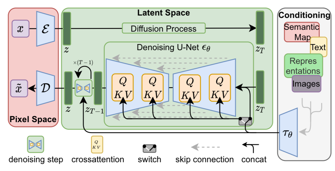
The above figure outlines the overall architecture of the conditional LDM demonstrated in the paper. Here, the crucial part to control the generated image is the conditioning mechanism, which is implemented by cross-attention. The encoder with condition can be denoted as $\mathcal{E}_\theta(z_t, t, y)$ where $y$ is the condition, which can either be text, semantic maps, or other image inputs.
As shown in the figure, the condition $y$ first passes through a network $\tau_\theta$ to be mapped to the latent space. The resulting $\tau_\theta(y)$ is fed into the attention modules that composes up the denoising UNet. In detail, each attention layer in the UNet uses $\tau_\theta(y)$ as the key($K$) and the value($V$), where the intermediate outputs of the UNet are utilized as the query($Q$), that is,
$$Q = W_Q^{(i)}\cdot \phi_i(z_t),$$
$$K = W_K^{(i)}\cdot \tau_\theta(y),$$
$$V = W_V^{(i)}\cdot \tau_\theta(y)$$
Considering that the projection of a vector $v$ onto the span of column vectors of $W$ (where the column vectors of W are unit vectors) is formulated by
$$\text{proj}_W(\mathbf{u}) = (\mathbf{u}^T W)W$$
This is roughly equivalent to the projection of UNet representations to the space determined by the input condition.
Putting this all together, the training objective can be expressed as
$$L_{LDM} = \mathbb{E}_{z\sim \mathcal{E}(x), y, \epsilon \sim\mathcal{N}(0, I), t}\left[\lVert \epsilon - \epsilon_\theta(z_t, t, \tau_\theta(y))\rVert_2^2\right]$$
where $\tau_\theta$ and $\epsilon_\theta$ are jointly optimized.
Experiments
The authors have conducted a number of experiments to study the adaptation of LDM on various tasks.
Downsampling Factor
First, the authors conducted an experiment varying the value of downsampling factor $f\in{1, 2, 4, 8, 16, 32}$, each of which the authors refer to as LDM-$f$. The paper reports that there is the trade-off between the training time and the fidelity of generated image over $f$.
Too small value of $f$ is bound to make the training process slow, while too large values can incur an excessive information loss, resulting in the low quality. LDM-4 and LDM-8 are considered as a reasonable choice between this trade-off.
Image Generation
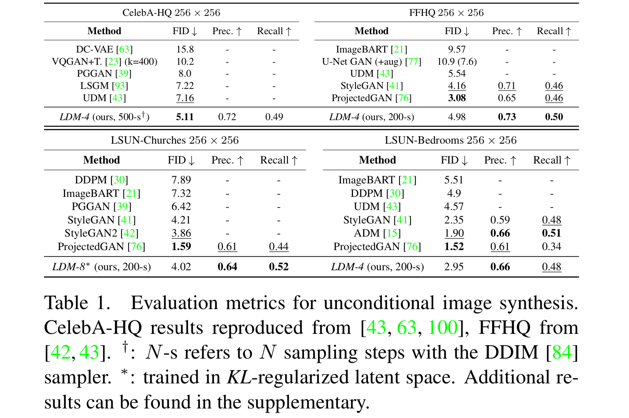
The authors then evaluated the (1) sample quality and (2) their coverage of the data manifold. For the latter, FID(Frechet Inception Distance) and Precision-and-Recall were used. Evaluating the metrics on four different datasets, LDM showed the best performance in the majority of cases, including CelebA-HQ, where the model achieved a new SOTA FID. Especially, LDM consistently showed the precision and recall better than GAN models, indicating that it has a wider mode coverage.
Note: How do we evaluate the precision and recall of a generative model?
The precision and the recall of the generative vision model represents how realistic and how diversified the generated images are, respectively. One way to assess these (Kynkäänniemi et al., 2019) is to embed the dataset images using a pre-trained VGGNet, approximate the manifold of real images using k-nearest neighbor (k-NN), and evaluate the precision and the recall by determining if the generated images are included in the learned manifold.
Conditional Image Generation
There are two ways in controlling the generation process of LDM: one using the cross-attention as described above, and the other held by concatenating the conditioning image to the input of denoising UNet.
Cross-Attention Based Conditioning
The authors apply cross-attention based conditioning on three types of tasks: (1) text-to-image, (2) semantic layout, and (3) ImageNet class condition.
Firstly, the authors trained a KL-reg LDM conditioned on the transformer output which embeds the text input to the latent space LDM uses.
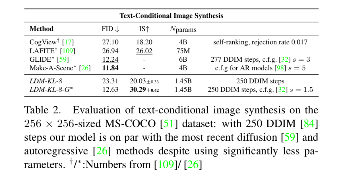
As depicted in the above table, the guided LDM-KL-8-G was on par with the SOTA autoregressive model, whie employing a significantly less number of parameters.
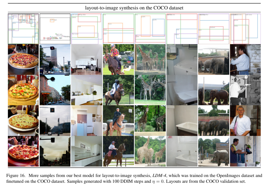
Secondly, the LDM was trained to synthesize images based on semantic layouts on COCO, performing layout-to-image synthesis. Below are the samples of generated images.
Finally, the authors conditioned LDM to synthesize images that correspond to each class of ImageNet. The results showed that LDM outperforms the SOTA LDMs can be conditioned by feeding the conditioning information together with the input of denoising UNet. Note that the image must be spatially aligned to be utilized as a condition.
Concatenation of Conditioning Image
Another way of controlling the image generation is to concatenating the spatially aligned conditioning image to the input of denoising UNet $\epsilon_\theta$. LDMs can thereby serve as image-to-image translation models. The authors apply this method into three tasks: (1) semantic synthesis, (2) super-resolution, and (3) inpainting.
Firstly, in the semantic synthesis, the images paired with corresponding semantic map were used to train the LDM. The downsampled version ($f=4$) of semantic map was fed to the diffusion model to generate the image.
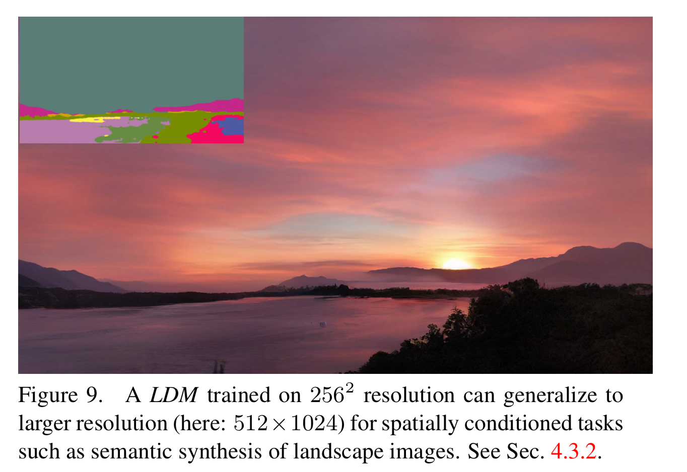
While experimenting for semantic synthesis, the authors discovered that the model generalizes well to a larger dimension. This is enabled by the convolution-based structure of the denoising UNet, which is insensitive to the input dimension, although it was trained on $256^2$. This feature was further applied to the super resolution and inpainting task, which are discussed in the continuing sections.
Super-Resolution
LDMs could effectively handle the super-resolution task by generating a high resolution image, conditioned on the low resolution version of it. The authors trained the model to restore the original image based on the image degraded via bicubic interpolation.
Although LDM did not succeed to outperform existing models in quantitative metrics, these metrics are known not to align with human-perceived quality. Human evaluation results show that LDM has a better performance in super-resolution.

Inpainting
Inpainting is a task where the model is trained to fill the masked region of the image. The authors have compared the LDM’s performance on the task with the SOTA approaches.
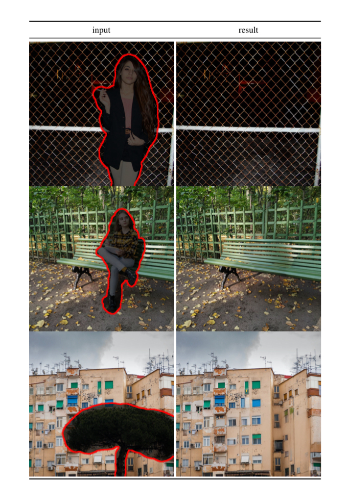
As the above figures indicate, LDMs showed a surprisingly good performance in inpainting.
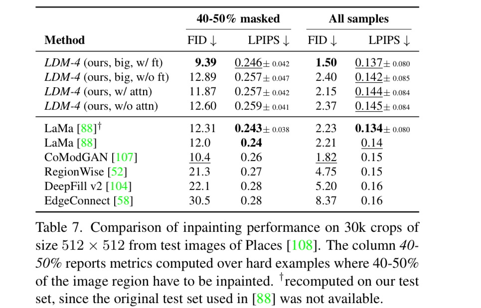
The quantitative results also suggests that LDM improves FID by a factor of at least 1.6x, while also reducing the time consumption.
Conclusion
In this paper, the authors have suggested a new methodology for generating images, stable diffusion. By introducing an autoencoder model to map the data to the latent space, on which the diffusion models are run, the authors could drastically reduce the computational demand while maintaining the image quality. The model allows various, multi-modal conditioning mechanisms to be applied, including text, class, and image. Through this general conditioning, the authors could apply the model into various downstream tasks, yielding the performance better than or at least on par of task-specific SOTA models.