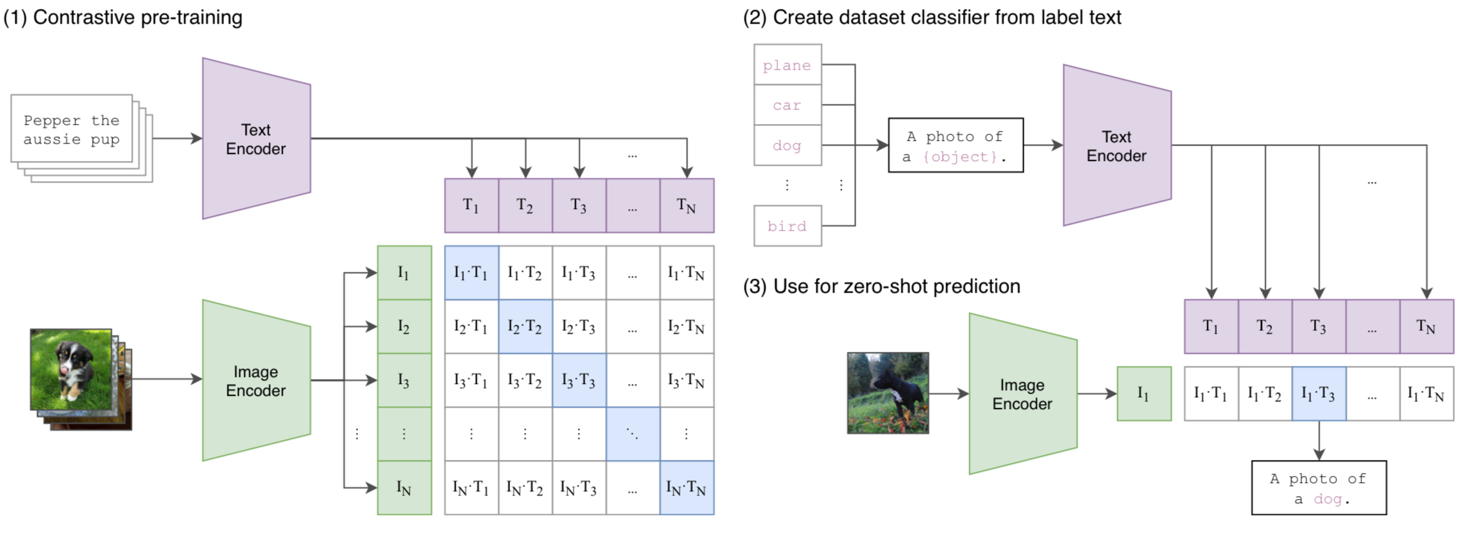
Radford, Alec, et al. "Learning transferable visual models from natural language supervision." International conference on machine learning. PMLR, 2021.
Background
Before the advent of CLIP, SOTA vision models were trained to predict the class of image within the fixed set of categories. This restricted both the generality and usability of the models, since they needed additional labelled datasets in order to learn a new visual concept.
In contrast, in the field of NLP, applying a pre-trained, task-agnostic models have already been a dominating approach. For example, GPT-3 have shown competitive results across many tasks, where the data were fed into the model in the standardized text-to-text manner. This indicates that it is better to train a model on a web-scale corpus with aggregate supervision than doing so with crowd-labelled datasets. Nevertheless, the vast majority of vision models still were trained on crowd-labelled datasets, e.g. ImageNet. Consequently, there has been multiple research on training vision models based on web text:
- Joulin et al. and Li et al. trained models to predict a word or n-grams in the caption based on the image.
- VirTex adopted a contrastive objective, which joinly trains the image and language models, and demonstrated the potential of its approach in learning image representations from text.
However, these model still underperformed the SOTA vision models, mainly because of their meager dataset scale. This is where CLIP, short for Contrastive Language-Image Pre-training, has come into the play, closing this performance gap by training model on large scale datasets. CLIP turns out to perform well on wide range of tasks, being even more robust and computationally efficient compared to ImageNet-supervised models.
Method
Creating a Sufficiently Large Dataset
Existing works training image models with natural language were restrained with their size of datasets. Compared to ResNeXt, which boasts the dataset with 3.5 billion instagram photos, existing approaches utilized datasets such as MS-COCO, Visual Genome, and YFCC100M. Excluding the images without proper descriptions have commonly resulted in the set with only about 15 million images, which is on par with ImageNet.
In this paper, the authors collected large quantity of publicly available images to construct a new dataset of 400 million text-image pairs. This comprises classes of about 20 thousand images, where each class collecting pairs with their text including one of 500 thousand queries. This is to diversity the set of visual concepts included in the dataset, which the author refer to as WeblmageText, of WIT.
Selecting an Efficient Pre-Training Method
At first, the authors attempted to predict the caption based on the image, as prior works did. However, the method struggled in scaling up. Finally, the alternative approach of contrastive learning was adopted, in which the model is trained to predict which text should be paired with which image.
To elaborate, CLIP employs two encoders, each for image and text, to map both domains to the multi-model embedding space. Each encoder extracts features from images and texts, and the resulting features passes through an additional linear layer to match the dimensions. The encoders are jointly trained to maximize the cosine similarity of the image and the text in the $N$ correct pairs, while minimizing that of $N^2-N$ incorrect pairs. This is done by
symmetric cross-entropy loss. Below is the numpy-style pseudocode for calculating the loss.
# image_encoder - ResNet or Vision Transformer
# text_encoder  - CBOW or Text Transformer
# I[n, h, w, c] - minibatch of aligned images
# T[n, l]       - minibatch of aligned texts
# W_i[d_i, d_e] - learned proj of image to embed
# W_t[d_t, d_e] - learned proj of text to embed
# t             - learned temperature parameter
# extract feature representations of each modality
I_f = image_encoder(I) #[n, d_i]
T_f = text_encoder(T)  #[n, d_t]
# joint multimodal embedding [n, d_e]
I_e = l2_normalize(np.dot(I_f, W_i), axis=1)
T_e = l2_normalize(np.dot(T_f, W_t), axis=1)
# scaled pairwise cosine similarities [n, n]
logits = np.dot(I_e, T_e.T) * np.exp(t)
# symmetric loss function
labels = np.arange(n)
loss_i = cross_entropy_loss(logits, labels, axis=0)
loss_t = cross_entropy_loss(logits, labels, axis=1)
loss   = (loss_i + loss_t)/
The code first calculates the $ \times n$ matrix of cosine similarities between all pairs,
logits. After that, it calculates the cross entropy loss two times:
- loss_i is the CE loss considering the images as the class, averaged between the texts
- loss_t is the CE loss calculated vice versa.
The final loss is calculated by taking average between the two cross entropy losses, which is why the loss is dubbed symmetric cross entropy. Since minimizing the cross entropy encourages the logit of the label class while discouraging other classes, this is a good proxy of the pairing task. Under this objective, CLIP is trained from scratch without using any pretrained parameters. Also, the temperature parameter is optimized together with the model, reducing the dimension of hyperparameter tuning.
Choosing and Scaling Model
Image Model
For the image encoder, ResNet and Vision Transformer(ViT) were used. ResNet has undergone three modifications, in which you can find the code here.
- The changes in ResNet-D were applied.
- Rect-2 blur pooling was introduced for anti-aliasing.
- The global average pooling was replaced with QKV attention pooling, where the query was conditioned on the global average-pooled result.
As for ViT, the original implementation was closely followed except for the additional layer normalization held after the addition of positional embeddings [code].
Text Model
Transformer architecture as in GPT-2 was introduced as the text model. The input sequences were tokenized using Byte Pair Encoding(BPE) representation, surrounded by special tokens [SOS] and [EOS]. The output from the [EOS] token was extracted as the feature representation of the overall sequence, after being passed to LayerNorm and linear projection.
Scaling Models
An EfficientNet-style scaling methods were used to scale the width, depth, and resolution of the image model at the same time. In contrast, text models were not scaled since they were regarded as less important for the performance than image models are.
As a result, five ResNets and three ViTs were trained:
- ResNet50, ResNet101, and three more scaled models with approximately 4x, 16x, and 64x compute of ResNet50, dubbed as RN50x4, RN50x16, and RN50x64.
- ViT-B/32, ViT-B/16, ViT-L/14.
Additionally, ViT-L/14 was trained for one additional epoch at a higher pixel size of 336px, following the approach suggested in FixRes. This model, ViT-L/14@336px, which turned out to perform the best, was used unless specified otherwise.
Note: The FixRes paper addresses the discrepancy between the domains of train and test set data. It argues that the differences in the crop methods during training and testing leads into a performance drop. Many models randomly crop the image after scaling up to 224px at train time, while they center crop at test time. To tackle this issue, the paper suggests fine-tuning the model after the training, by replacing the FC layer after the AvgPool.
Using CLIP
The authors applied CLIP to downstream tasks and studied its capability of zero-shot transfer by evaluating it on standard vision datasets. In each of the datasets, they conducted the classification task by using the class labels as text entities to be matched with the images. The also engaged in prompt engineering, such as matching a cat image not with the text “a cat,” but with the sentence “This is a cat.” Additionally, they experimented with ensembling results from various prompts.
Experiments
Comparison to Visual N-Grams
Visual N-Grams is the first paper which studied the zero-shot transfer to existing image datasets.

As the above table indicates, CLIP outperformed Visual N-Grams with a great margin, achieving performance on par with fully supervised models. Note that the comparison was held for models that can be trained within a GPU day.
The authors extend the meaning of zero-shot learning, which usually refers to “generalizing to unseen object categories,” into generalization to unseen datasets. By assessing the zero-shot performances, the authors studied the task learning capability of CLIP.
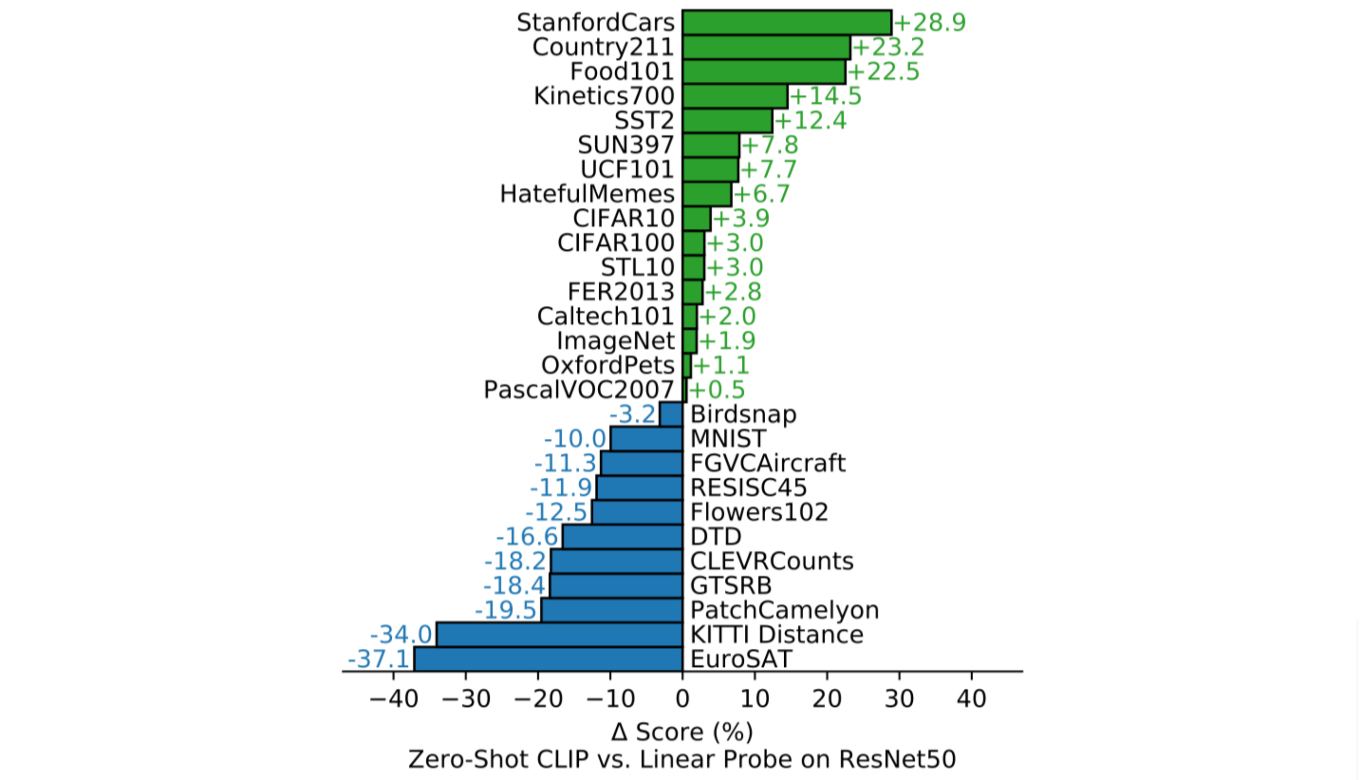
The above graph depicts the performance difference between CLIP and ResNet50 on linear probe across 27 datasets. As the graph ascends, it signifies that CLIP exhibited relatively higher performance compared to ResNet50.
- On STL10, a dataset containing only a limited number of labelled examples, CLIP achieved a new SOTA performance.
- Among the fine-grained classification datasets, CLIP performed well on some of the tasks while struggling on others.
- CLIP did well on Stanford Cars and Food 101, while it did not on Flower102 and FGVCAircraft.
- The putative cause of the difference is the varying amount of per-task supervision between (CLIP’s) WIT and (ResNet50’s) ImageNet.
- On video action recognition, CLIP showed a superb performance, primarily due to its labels containing abundant verbs, while ImageNet comprises noun-centric visual concepts.
- CLIP underperformed on several specialized, complex, or abstract tasks.
- However, the authors point out that zero-shot transfer might not be a fair metric for some tasks that only experts can perform well, e.g. lymph node tumor classification. For these tasks, few-shot transfer may be more adequate.
Zero-Shot CLIP vs Few-Shot Linear Probes
To contextualize the zero-shot CLIP performance, the authors compared the model to few-shot methods.
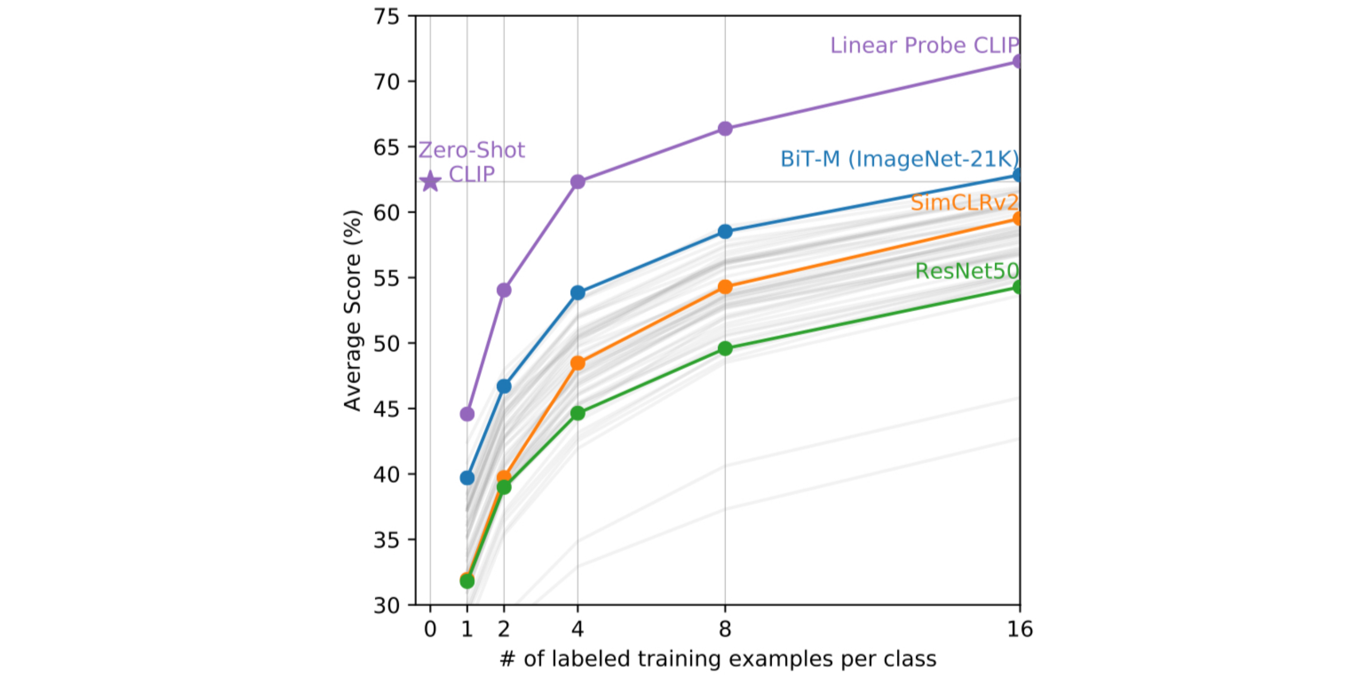
The above plot shows that zero-shot CLIP matches the performance of a 4-shot CLIP with linear probing, although one might expect even a one-shot model may outperform zero-shot CLIP. This is because while CLIP can directly specify visual concept through natural language, few-shot learners have to learn this indirectly through examples. This context-less example-based learning is prone to spurious correlations, especially in one-shot case.
Representation Learning
The authors used linear probing evaluation to study the representation learning performance.
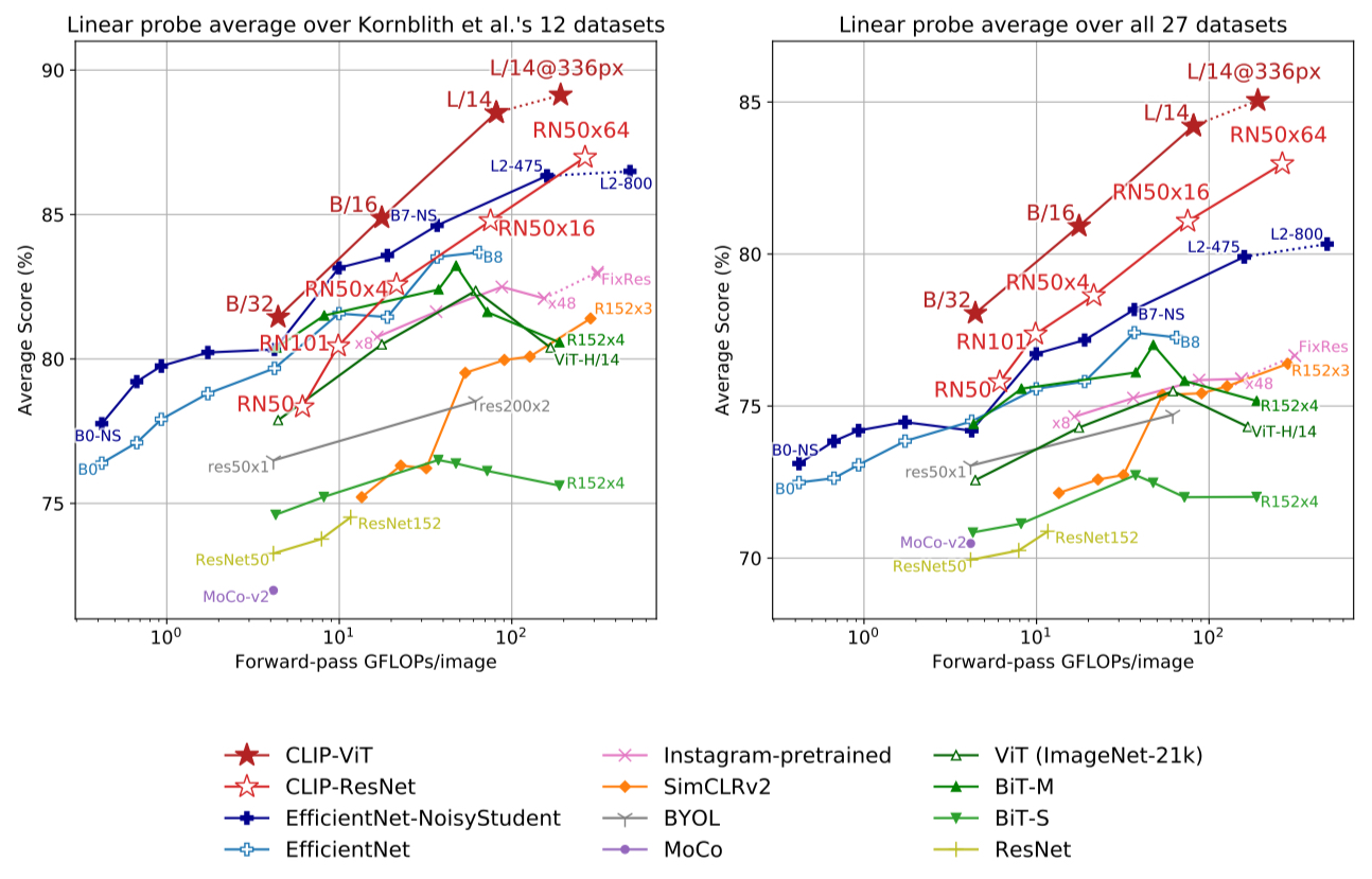
The results demonstrate that CLIP has the representation learning capacity even outperforming the best existing model. The gap even enlarges when the authors tested on the newly constructed suite of datasets, which resolves the bias towards ImageNet-like tasks.
Robustness to Distribution Shift
Finally, the authors evaluated the robustness of CLIP under distribution shifts. They did so by comparing Zero-shot CLIP to the models trained on ImageNet dataset, along with those trained with robustness techniques.
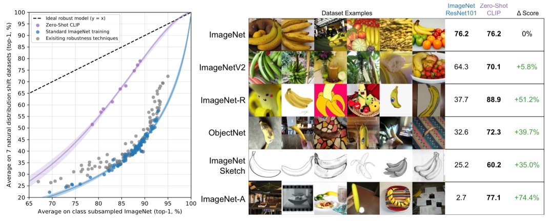
The plot demonstrates that Zero-shot CLIP shows a significantly better robustness to distribution shifts, where the images on the right panel shows the examples of images under the distribution shifts. This is due to the inherent nature of zero-shot learning, which does not rely on spurious correlations present only on a specific distribution.