Hu, Edward J., et al. "Lora: Low-rank adaptation of large language models." arXiv preprint arXiv:2106.09685 (2021).
Suggested by Microsoft, LoRA(Low-Rank Adaptation) is a powerful method in performing parameter-efficient fine-tuning (PEFT). This article delves into the method employed in LoRA and how it works to efficiently fine-tune an LLM. Furthermore, a code snippet for fine-tuning GPT-2 with LoRA using the built-in features of the Hugging Face Trainer class is included.
Introduction & Previous Work
Recently, most adaptations of LLM to a specific downstream task rely on fine-tuning. That is, the pre-trained weights are loaded and go through an additional few training steps on the task dataset. However, as larger language models are introduced, the cost for fine-tuning has also skyrocketed. For example, GPT-3 has 175 billion parameters, which cannot even be loaded to a single GPU. Therefore, there needs to be a solution to fine-tune a large language model efficiently.
A number of methods have been proposed to cope with this problem:
-
Adding adapter layers: an adapter layers can be added between the existing layers of a model. During the training, all other layers are frozen while the adapters become the only learnable layer.
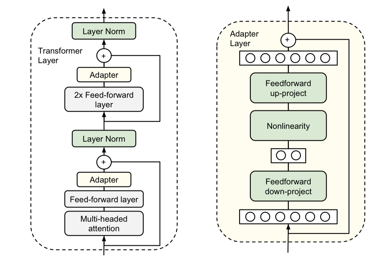
Houlsby et al. (2019)
Despite its effectiveness, this increases the latency since the sequential structure interferes with the parallelism the original model exploits.
-
Optimizing the Prompt: This line of work can be epitomized by prefix tuning, where an additional learnable vectors (dubbed the prefix) are prepended to the prompt. This reduces the trainable parameter significantly, since only the prefix vectors are updated during the fine-tuning step. However, these methods are known to be difficult to optimize, show non-monotonic performance change as the number of parameter increases. Also, the method necessarily reduces the sequence length since a number of tokens should be reserved for learnable prefix.
Method
The approach that the authors take is inspired by the observation of a previous work: the learned over-parametrized models in fact reside on a low intrinsic rank. The authors hypothesized that the changes in weights($\Delta W$) may also have a low rank, and exploit the hypothesis.
To be more specific, suppose that we have a pre-trained autoregressive language model $P_{\Phi}(y|x)$ parametrized by $\Phi$. When the model undergoes fine-tuning, the parameter changes from $\Phi$ to $\Phi+\Delta\Phi$ as the solution to the following optimization problem:
$$\max_{\Phi}\sum\limits_{(x, y)\in \mathcal{Z}}\sum\limits_{t=1}^{|y|}\log P_{\Phi}(y_{t}|x,y_{<t})$$
However, this generates a set of parameters $\Delta \Phi$ for every single downstream task, laying inefficiency. Therefore, a line of work has studied the way to parametrize $\Delta \Phi$ with another parameter, say $\Theta$. Thus, the optimization problem is transformed as below.
$$\max_{\Theta}\sum\limits_{(x, y)\in \mathcal{Z}}\sum\limits_{t=1}^{|y|}\log P_{\Phi+\Delta\Phi(\Theta)}(y_{t}|x,y_{<t})$$
The authors use a low-rank representation to encode $\Delta\Phi$. To do so, they trained two separate matrices in which the product is added to the pre-trained weight.
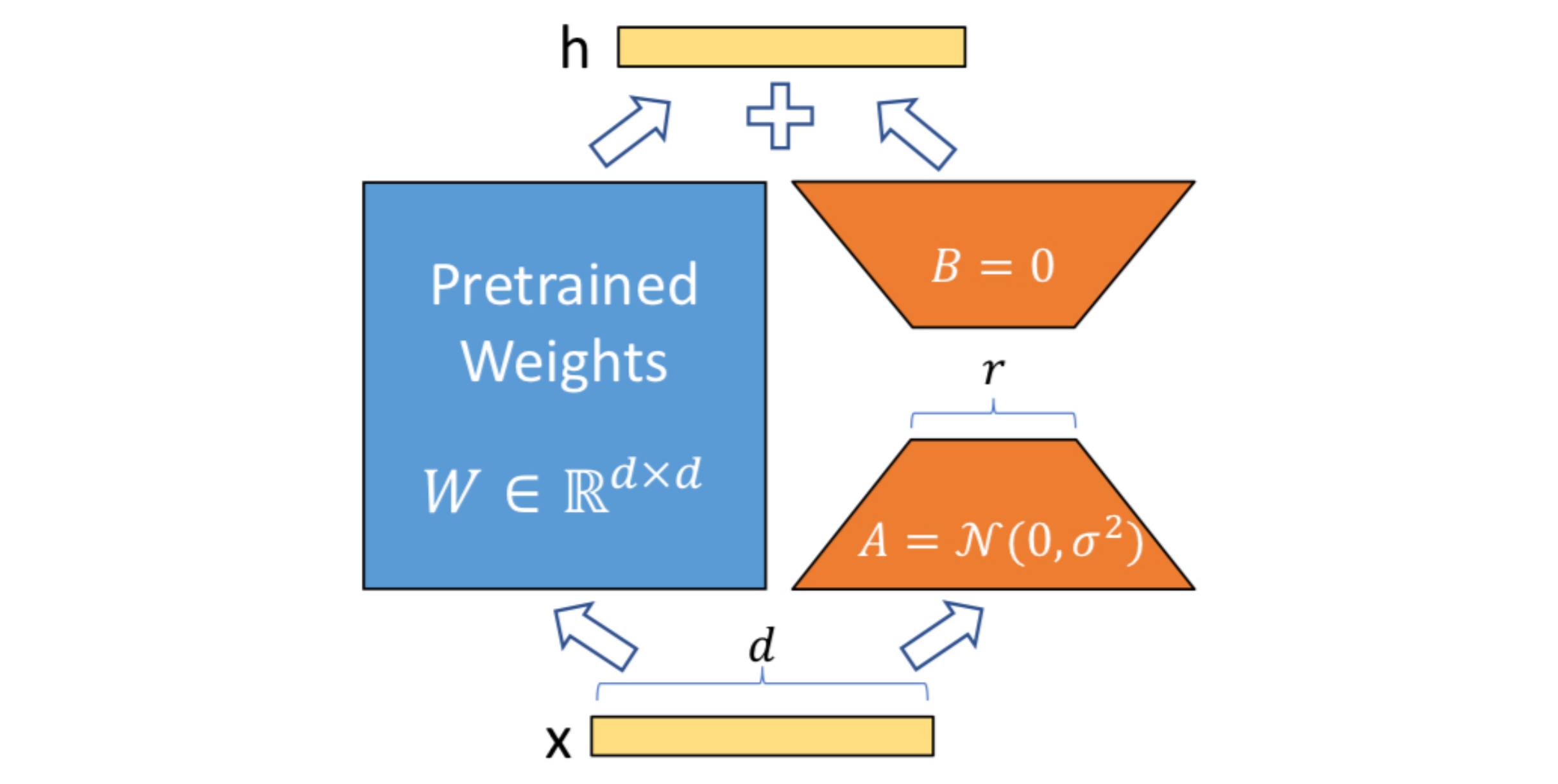
As depicted in the above figure, a layer with weight matrix $W\in\mathbb{R}^{d\times k}$ is replaced with $W+BA$, where $B\in\mathbb{R}^{d\times r}, A\in\mathbb{R}^{r\times k}$. During the training step, only the matrices $A$ and $B$ are learned, whereas the original matrix $W$ remains fixed. Here, $r$ is set to be much smaller than $d$ or $k$, thereby constraining the rank of $BA$ to be $r$. (Note that $d$ does not necessarily have to be same with $n$, although the figure describes otherwise.)
Note: Why is $\text{rank}(BA)=r$ ?
One of the definitions of the rank of a matrix is the number of linearly independent column vectors. Denoting the $r$ column vectors of $B$ as $\mathbf{b}_{1}, \mathbf{b}_{2}, \cdots, \mathbf{b}_r$,
$$BA=\begin{bmatrix}|&|&\cdots&|\\\mathbf{b}_1&\mathbf{b}_2&\cdots&\mathbf{b}_{r}\\|&|&\cdots&|\end{bmatrix}\begin{bmatrix}a_{11}& a_{12}&\cdots&a_{1k}\\ a_{21}& a_{22}&\cdots&a_{2k}\\\vdots&\vdots&\ddots&\vdots\\ a_{r1}& a_{r2}&\cdots&a_{rk}\ \end{bmatrix}$$
$$=\begin{bmatrix}a_{11}\mathbf{b}_1^T+a_{21}\mathbf{b}_2^T+\cdots+a_{r1}\mathbf{b}_r^T\\a_{12}\mathbf{b}_1^T+a_{22}\mathbf{b}_2^T+\cdots+a_{r2}\mathbf{b}_r^T\\\vdots\\a_{1k}\mathbf{b}_1^T+a_{2k}\mathbf{b}_2^T+\cdots+a_{rk}\mathbf{b}_r^T\end{bmatrix}^T$$
Therefore, the number of linearly independent column vectors is bound to be less than or equal to $r$. Since the elements of the matrix are randomly initialized and trained values, we can neglect the possibility that they match exactly to generate an additional linear dependency. Thus, $\text{rank}(BA)=r$.
Therefore, the modified forward pass becomes
$$h = W_{0}x+\Delta W x=W_0x+BAx$$
where the learnable matrices $A$ and $B$ are initialized with $\mathcal{N}(0, \sigma^2)$ and zero. In practice, the term for $\Delta Wx$ is scaled by $\alpha/r$. The authors mention that $\alpha$ performs a role similar to the learning rate, and fixing its value to be same to the initial value of $r$ reduces the further need for hyper-parameter tuning.
LoRA has several advantages over existing methods:
- It easily generalizes to full fine-tuning. To elaborate, increasing the value of $r$ sufficiently large makes the model converge to the full fine-tuning. In contrast, adapter-based models would converge to MLP and prefix-based model to that cannot take sequences long enough.
- It does not introduce additional latency. During the inference time, the additional matrices $A$ and $B$ can be absorbed to the original model’s weight matrix: $W^\prime=W_0+BA$. Therefore, does not affect the latency at all.
Since transformers are the key components of state-of-the-art large language models, the authors mention how LoRA can be exploited in transformer modules. The authors applied the adaptation matrices $A$ and $B$ only to the attention weights $W_{q}, W_k,W_v$, and $W_o$, while parameters in MLP remain frozen, inducing both the simplicity and parameter-efficiency.
Applying the LoRA to transformer-based models has following advantages:
- It reduces VRAM consumption during the training by almost 2/3.
- The checkpoint size is reduced by roughly 10000, since only the low-rank adaptation matrices are saved.
- Also, switching between the tasks becomes much simpler since only the adaptation matrices are replaced.
- Lastly, training speed is increased by about 25%.
Experiments
The authors have evaluated LoRA on downstream tasks using a number of models: RoBERTa, DeBERTa, GPT-2, and GPT-3 175B. To contextualize the performance of LoRA, several baselines are evaluated at the same time:
- Classical Fine-tuning,
- Bias-only or BitPit, which trains only the bias part of the model while freezing the weights.,
- Prefix-embedding tuning (PreEmbed), which, as discussed previously, prepends trainable special tokens to the input sequence,
- and adapter tuning, which inserts a separate adapter unit between the layers.
Results
RoBERTa and DeBERTa
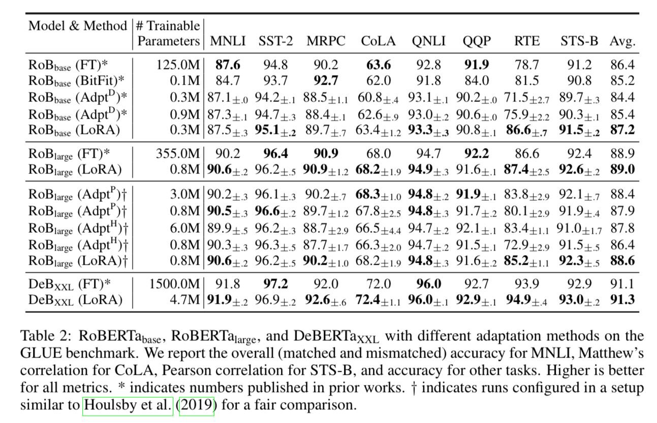
The authors measured the ability of NLU(natural language understanding) when fine-tuned with each method. The table above demonstrates the performance of RoBERTa and DeBERTa along with the number of trainable parameters. Training with LoRA showed the performance on par with, or even outperforming the full fine-tuning.
GPT-2
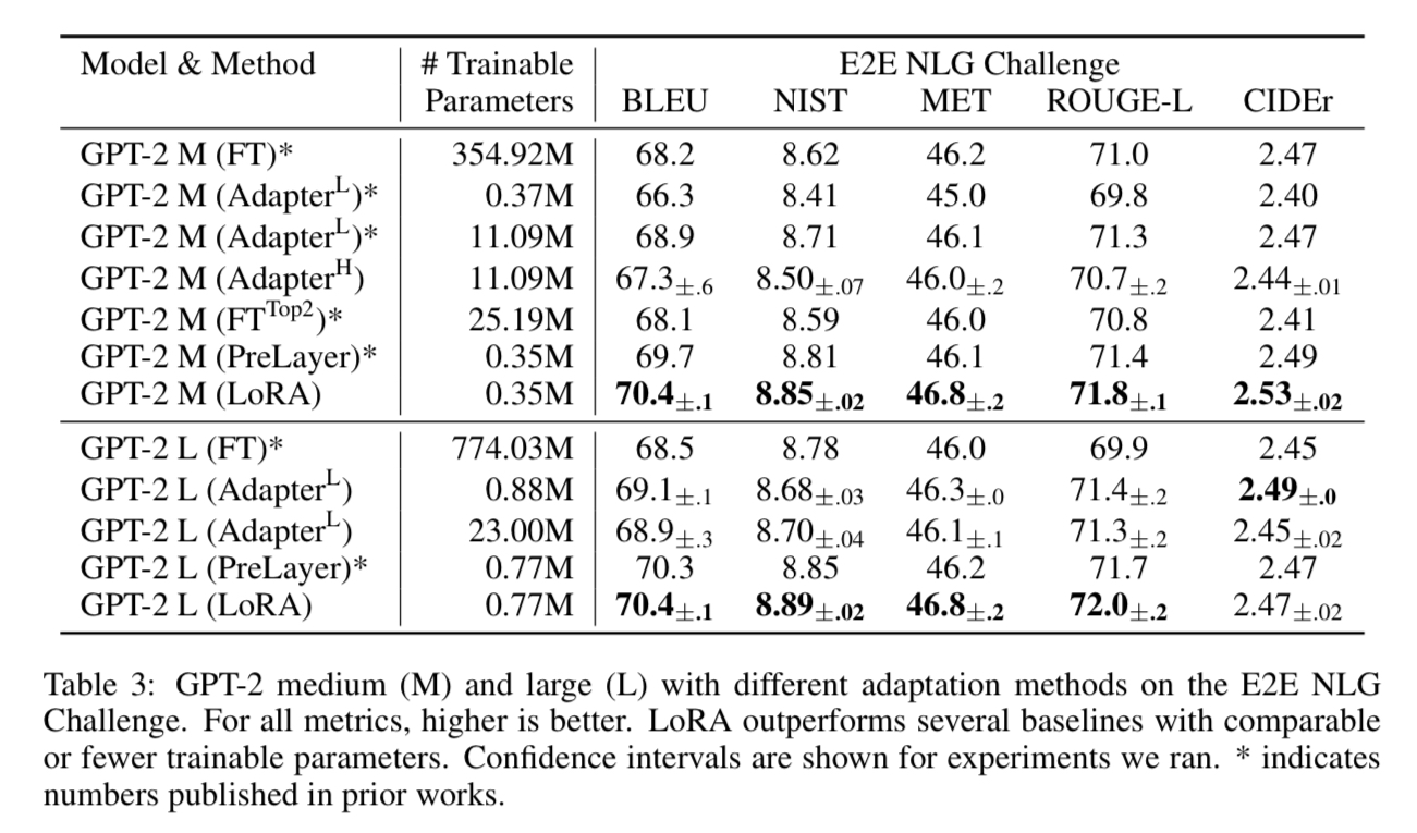
When training GPT-2 on E2E NLG(End-to-End Natural Language Generation) task, LoRA consistently delivered the best performance with only one exception, while drastically reducing the number of trainable parameters.
GPT-3
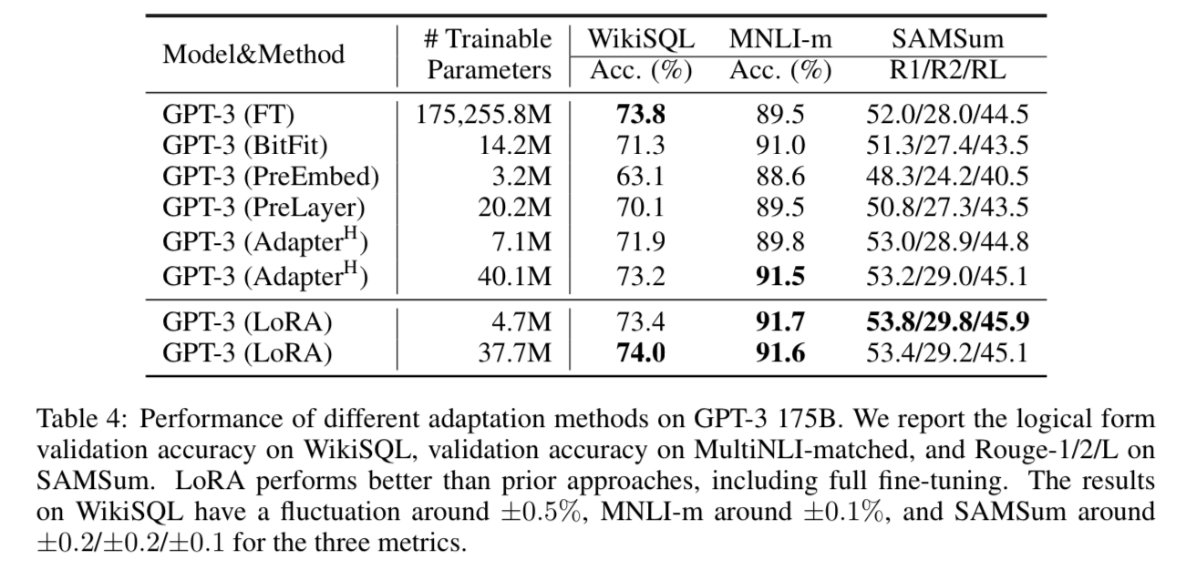
Finally, the authors scaled up to GPT-3 with 175 billion parameters. As in the table, LoRA matched outperformed the classical fine-tuning baseline with all three tasks.
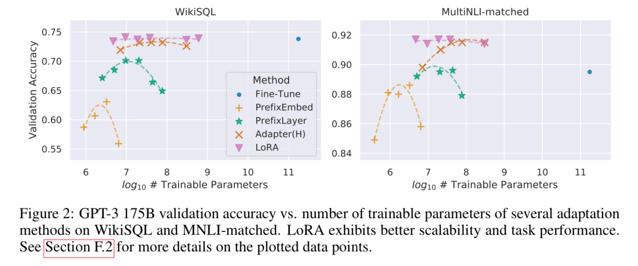
Figure 2 shows that LoRA’s performance is not only the best, but also consistent when faced scale-up. In contrast, other methods, especially prefix-based methods, demonstrated a performance drop when the number of parameters increased.
Understanding the Low-Rank Updates
To answer the following questions, the authors have conducted a series of empirical studies:
- Given the restriction in the number of parameters, which subset of weights should we adapt to maximize the fine-tuning performance?
- Is the optimal $\Delta W$ actually rank-deficient?
- How is $\Delta W$ correlated with the original $W$?

First, the authors applied LoRA to different subsets of transformer weights, varying the rank $r$ to match the total number of parameters roughly. The results show that it is better to adapt LoRA to all weight matrices: $W_q, W_k, W_v$, and $W_o$, in an attention module, even if we need to adjust the rank $r$ to be as low as 2. In contrast, putting all the parameters to $W_q$ or $W_k$ showed a significant performance drop.
What is the Optimal Rank?
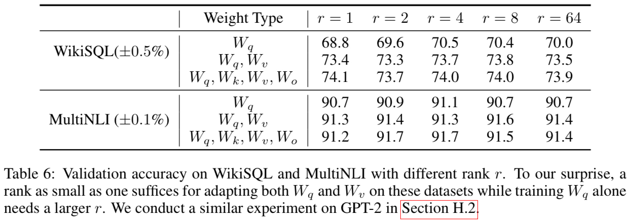
The authors experimented with varied values of $r$, in order to find the optimal rank. According to the results, the performance stagnated as $r$ exceeds 4. The surprising part in the result was that using a very small value of $r$ ($r=$ 1 or 2) still showed a competitive performance. This indicates the weight update $\Delta W$ has very small intrinsic rank and thus increasing $r$ does not allow the model to discover a meaningful additional subspace. Therefore, a low-rank matrix is sufficient for adaptation.
To support this finding, the authors measured the subspace similarity between different $r$ choices, using the Grassmann distance. This is to answer the following question:
How much of the subspace spanned by the top $i$ singular vectors in $U_{A_{r=8}}(1\le i\le 8)$ contained in the subspace spanned by top $j$ singular vectors of $U_{A_{r=64}}(1\le j\le 64)$?
This was done by obtaining the singular value decomposition (SVD) of adaptation matrices $A_{r=8}$ and $A_{r=64}$ from the same pre-trained model and yielding the right-singular unitary matrices $U_{A_{r=8}}$ and $U_{A_{r=64}}$, which were put into the following formula:
$$\phi(A_{r=8}, A_{r=64}, i, j) = \frac{\lVert {U_{A_{r=8}}^i}^TU_{A_{r=64}}^j\rVert_F^2}{\min(i, j)}\in[0, 1]$$
Where $U_A^i$ denotes the columns of $U_A$ corresponding to the top-$i$ singular vectors. Here, $\phi=1$ represents a complete overlap of subspaces, where $\phi=0$ a complete separation. The authors plot the values of $\phi$ with all the combinations of $i$ and $j$.
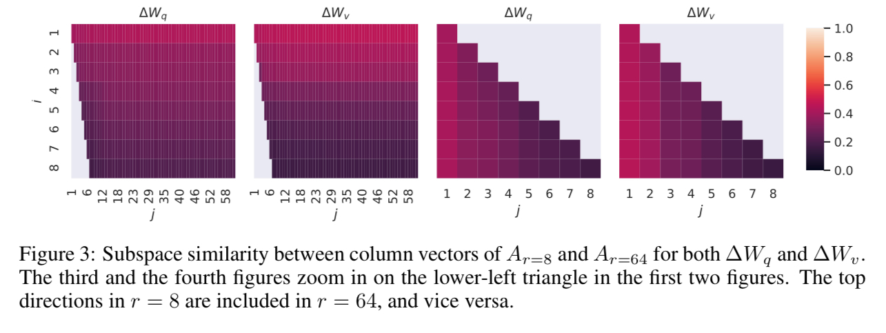
From the plots above, the authors could deduce that the top singular vectors of $A_{r=8}$ and $A_{r=64}$ overlaps significantly. Also, the subspace of dimension 1 had the normalized similarity exceeding 0.5, which explains why even $r=1$ works well in the downstream tasks.
How Does the Adaptation Matrix $\Delta W$ Compare to $W$?
Finally, the authors studied the correlation between $\Delta W$ and $W$. Also, they have investigated the magnitude of $\Delta W$ to see if they are large enough to change the directions of $W$ significantly.
To do so, the authors projected $W$ onto the $r$-dimensional subspace of $\Delta W$. This was done by extracting the left and right singular matrices from the SVD of $\Delta W$, and applying $U^TWV^T$. The Frobenius norms $\lVert U^TWV^T\rVert_F$ and $\lVert W\rVert_F$.

The results suggest several facts:
- $\Delta W$ has a significant correlation with $W$. Thus, $\Delta W$ amplifies some features in $W$.
- The subjects of such amplification are mostly the features that are not represented enough in $W$.
- The amplification factor is rather huge. For $r=4$, it amplified the features by multiple of $6.91/0.32 \approx 21.5$ in average.
Thus, the authors could conclude that low-rank adaptations amplify the features that are important in a specific downstream task, which are already present but not emphasized in the pre-trained model .
LoRA can be easily applied to fine-tuning task using the peft library, which works on Hugging Face transformers library. In this section, we will be fine-tuning a GPT-2 on IMDb dataset with LoRA. The components irrelevent with LoRA are based on this article (Korean).
Install Required Libraries
%%capture
!pip install -U datasets transformers accelerate peft
Prepare Model and Tokenizer
from transformers import AutoTokenizer, AutoModelForSequenceClassification

model_ckpt = "openai-community/gpt2"
tokenizer = AutoTokenizer.from_pretrained(model_ckpt)
model = AutoModelForSequenceClassification.from_pretrained(model_ckpt)

model.config.pad_token_id = tokenizer.eos_token_id
tokenizer.pad_token_id = tokenizer.eos_token_id
Load the model and the tokenizer from transformers. Also, set the pad token to be the EOS(end of sequence) token.
Select the Target Modules
To set the target to which LoRA will be applied, we use the following code to list the named modules contained in the model.
for name, module in model.named_modules():
    print(name)
transformer
transformer.wte
transformer.wpe
transformer.drop
transformer.h
transformer.h.0
transformer.h.0.ln_1
transformer.h.0.attn
transformer.h.0.attn.c_attn
transformer.h.0.attn.c_attn.base_layer
transformer.h.0.attn.c_attn.lora_dropout
transformer.h.0.attn.c_attn.lora_dropout.default
transformer.h.0.attn.c_attn.lora_A
transformer.h.0.attn.c_attn.lora_A.default
transformer.h.0.attn.c_attn.lora_B
transformer.h.0.attn.c_attn.lora_B.default
transformer.h.0.attn.c_attn.lora_embedding_A
transformer.h.0.attn.c_attn.lora_embedding_B
transformer.h.0.attn.c_proj
transformer.h.0.attn.c_proj.base_layer
transformer.h.0.attn.c_proj.lora_dropout
transformer.h.0.attn.c_proj.lora_dropout.default
transformer.h.0.attn.c_proj.lora_A
transformer.h.0.attn.c_proj.lora_A.default
transformer.h.0.attn.c_proj.lora_B
transformer.h.0.attn.c_proj.lora_B.default
transformer.h.0.attn.c_proj.lora_embedding_A
transformer.h.0.attn.c_proj.lora_embedding_B
transformer.h.0.attn.attn_dropout
transformer.h.0.attn.resid_dropout
...
By looking at the module list, you can determine that the target for LoRA should be set to transformer.h.*.attn.c_*. We will use a regular expression to specify the modules with such name.
from peft import LoraConfig, get_peft_model

config = LoraConfig(r=4, target_modules='transformer\.h\..*\.attn\.c_.*')
model = get_peft_model(model, config)
model.print_trainable_parameters()
trainable params: 221,184 || all params: 124,662,528 || trainable%: 0.17742621102629974
This is a main part of the code where LoRA is applied. By applying rank-4 adaptations to modules with specified names, we could reduce the number of trainable parameters to only 0.177% of the full model.
Prepare the Dataset
from datasets import load_dataset
dataset = load_dataset("stanfordnlp/imdb")

def tokenize(batch):
    tokenized = tokenizer(batch["text"], max_length=256, truncation=True, padding=True)
    return {"input_ids": tokenized["input_ids"], "attention_mask": tokenized["attention_mask"]}


ds_train = dataset['train'].shuffle().select(range(10000))
ds_test = dataset['test'].shuffle().select(range(2500))

ds_train = ds_train.map(tokenize, batched=True)
ds_test = ds_test.map(tokenize, batched=True)
Load the IMDb dataset from transformers, and tokenize to transform it into a form that model can accept. Note that we only use a subset of the original IMDb dataset.
Define Metrics
import numpy as np
from datasets import load_metric
from transformers import TrainingArguments, Trainer

accuracy_metric = load_metric("accuracy")
f1_metric = load_metric("f1")

def compute_metrics(eval_pred):
    predictions, label_ids = eval_pred.predictions, eval_pred.label_ids
    predictions = predictions.argmax(axis=1)
    accuracy = accuracy_metric.compute(predictions=predictions, references=label_ids)
    f1 = f1_metric.compute(predictions=predictions, references=label_ids, average="weighted")

    return {
        "accuracy": accuracy["accuracy"],
        "f1": f1["f1"],
    }
The compute_metrics function is defined in the way suggested in the previous article (Korean). It calculates the metrics that are used for evaluation.
Training
from transformers import Trainer, TrainingArguments

training_arguments = TrainingArguments(
    output_dir='./results',
    evaluation_strategy="epoch",
    num_train_epochs=10,
    per_device_train_batch_size=32,
    per_device_eval_batch_size=32,
    learning_rate=1e-3,
    weight_decay=1e-5,
    logging_strategy="epoch",
    load_best_model_at_end=True,
    save_strategy="epoch",
    metric_for_best_model="accuracy",
    report_to="none"
)

trainer = Trainer(
    model=model,
    train_dataset=ds_train,
    eval_dataset=ds_test,
    args=training_arguments,
    compute_metrics=compute_metrics,
)
trainer.train()
Finally, we perform training by using the Trainer API.
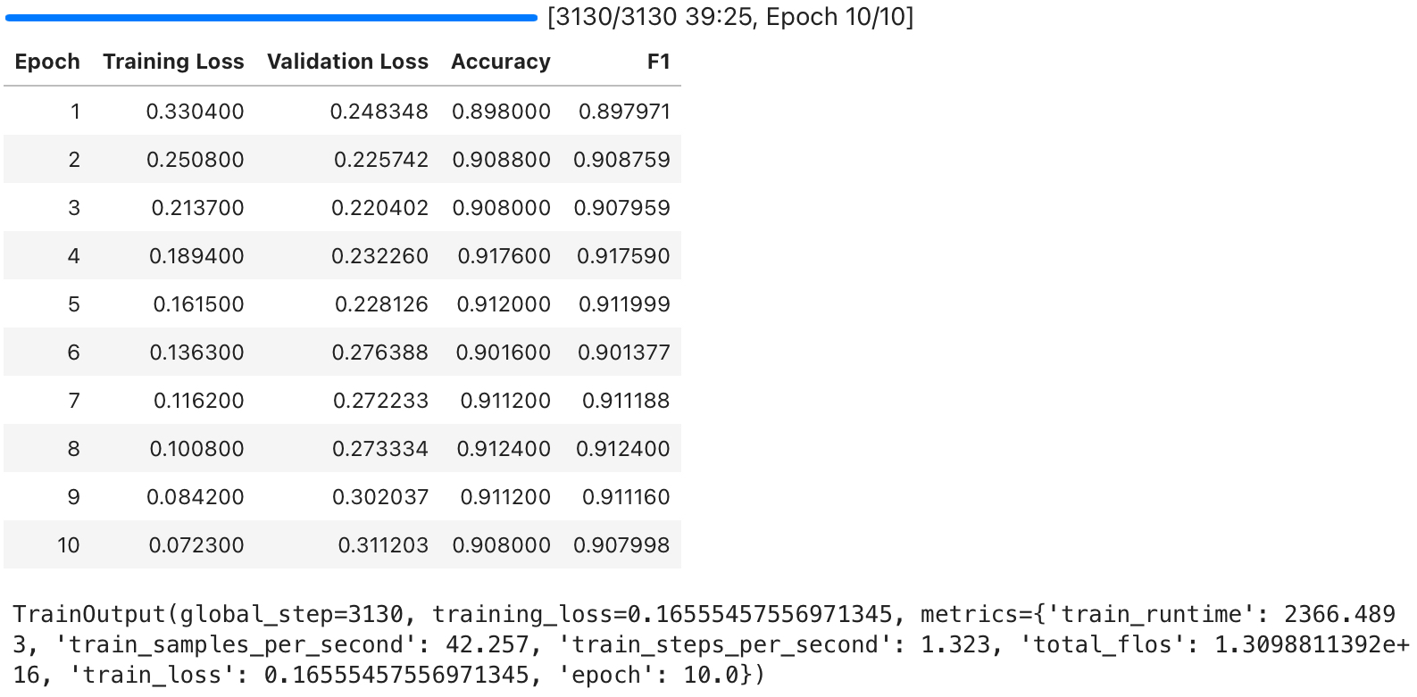
The result shows that the training has progressed well.