
Chen, Tianqi, and Carlos Guestrin. "Xgboost: A scalable tree boosting system." Proceedings of the 22nd acm sigkdd international conference on knowledge discovery and data mining. 2016.
XGBoost(Extreme Gradient Boosting) is a scalable, efficient machine learning technique applicable to data in table format. The model can be applied for both the classification and the regression task, winning 17 out of 29 Kaggle challenges .
Introduction
Despite the recent success of deep learning models, mainly powered by CNN or transformer architectures, there still are fields were classical machine learning models are needed. This includes the processing of data in the table form, where each entry comprises a number of feature values. Since handling these data usually involves one of two tasks -- classification and regression -- a powerful and efficient machine learning model is required.
XGBoost utilizes tree boosting to tackle these tasks. It outperforms classical approaches by great margin, including linear regression. Also, its awareness of scalability and sparsity allows the processors to accomplish these tasks efficiently. Finally, XGBoost engages in parallelism, distributed computing, and out-of-core computing to optimize the performance.
In the following sections, I will briefly go through the theoretical background and the implementation of XGBoost.
Tree Boosting in a Nutshell
This section summarizes how the existing tree boosting algorithm works, from which the XGBoost is derived.
The Objective
Given the dataset $\mathcal{D}={(\mathbf{x}_i, y_i)}$, where $|\mathcal{D}| = n$, $\mathbf{x} \in\mathbb{R}^m$, and $y_i\in\mathbb{R}$, a tree ensemble model uses $K$ different trees where the results of each are added to estimate the output $y_i$:
$$ \hat{y}_i = \phi(\mathbf{x}_i) =\sum\limits_{k=1}^{K}f_k(\mathbf{x}_i), \quad f_{k}\in\mathcal{F}$$
Here,
$$\mathcal{F}={f(\mathbf{x})=w_{q_{(\mathbf{x})}}}$$
denotes the space of regression trees, where $q:\mathbb{R}^m \to T$($T$: number of leaves) represents the structure of the tree. The weight $w_i$ is a number attached to the leaf node $i$.
Thus, when a tree evaluates an instance, the function $q$ maps the input instance to the leaf node $q(\mathbf{x})$, and the weight that corresponds to the leaf, $w_{q(\mathbf{x})}$, is returned as the output. The system is called an ensemble since it utilizes a number of trees and combines the return value of each trees to yield the final result.
To train a tree ensemble model, we must devise an objective function for it. The function can simply be formulated as follows:
$$\mathcal{L}(\phi) = \sum\limits_i l(\hat{y}_i, y_i) +\sum\limits_k \Omega(f_k)$$
where the regularization term $\Omega(f) = \gamma T + \frac{1}{2}\lambda \lVert w \rVert^2$ is added to a convex, differentiable loss function $l$.
Gradient Tree Boosting
Then how do we optimize the discrete structure of forest with such a differentiable objective? To accomplish this, the authors decide to optimize the model in an additive manner. Thus, a new tree is added to minimize the loss function, on top of the set of already included set of trees. Formally, during the iteration $t$, a new tree $f_t$ must be added to optimize
$$\mathcal{L}^{(t)} = \sum\limits_{i=1 }^n l(y_i, \hat{y}_i{(t-1)} + f_t(\mathbf{ x}_i)) +\Omega(f_t)$$
Since it is difficult to directly optimize the above function, we take the second order approximation of $1$ with respect to $f_t(\mathbf{x})$:
$$\mathcal{L}^{(t)} \approx \sum\limits_{i=1}^n [ l(y_i, \hat{y}_i^{(t-1)}) + g_{i}f_t(\mathbf{x}_i) + \frac{1}{2} h_i f_t^2(\mathbf{x}_i)] + \Omega(f_t)$$
where
$g_i = \partial_{\hat{y}^{(t- 1)}} l(y_i, \hat{y}^{(t- 1)})$ and $h_i = \partial_{\hat{y}^{(t- 1)}}^2 l(y_i, \hat{y}^{(t- 1)})$ are the first and the second order partial derivatives of $l$. Dropping the constant terms and substituting $\Omega(f_t) = \gamma T + \frac{1}{2} \lambda \sum\limits_{j=1}^T w_j^2$ yields
$$\tilde{\mathcal{L}}^{(t)} =\sum_{i=1}^n\left[g_i f_t\left(\mathbf{x}_i\right)+\frac{1}{2} h_i f_t^2\left(\mathbf{x}_i\right)\right]+\gamma T+\frac{1}{2} \lambda \sum_{j=1}^T w_j^2$$
Additionally, we can group the instances by the leaf nodes each falls into. Let $I_j={i|q(\mathbf{x}_i)=j}$ be the input instances that are mapped to the leaf node $j$. Reorganizing the summation by $1 j$ gives the quadratic function of $w_i$'s,
$$=\sum_{j=1}^T\left[\left(\sum_{i \in I_j} g_i\right) w_j+\frac{1}{2}\left(\sum_{i \in I_j} h_i+\lambda\right) w_j^2\right]+\gamma T$$
where we can express the minimum value in closed-form:
$$\tilde{\mathcal{L}}^{(t)}(q)=-\frac{1}{2} \sum_{j=1}^T \frac{\left(\sum_{i \in I_j} g_i\right)^2}{\sum_{i \in I_j} h_i+\lambda}+\gamma T$$
which is attained when $w _j^\ast = -\frac{\sum_{i\in I_j} g_i}{\sum_{i\in I_j} h_i + \lambda}$.
Even using the above simplified objective, we still cannot evaluate all possible tree structures. Therefore, the optimization is held by deciding whether to partition the instance set of each leaf of not. When a leaf node with input instances $I$ is split by $I_L$ and $I_R$, the reduction in loss is given by
$$\mathcal{L}_{\text {split }}=\frac{1}{2}\left[\frac{\left(\sum_{i \in I_L} g_i\right)^2}{\sum_{i \in I_L} h_i+\lambda}+\frac{\left(\sum_{i \in I_R} g_i\right)^2}{\sum_{i \in I_R} h_i+\lambda}-\frac{\left(\sum_{i \in I} g_i\right)^2}{\sum_{i \in I} h_i+\lambda}\right]-\gamma$$
This serves as the criterion of choosing the partition that maximizes the gain.
Overfitting Prevention: Shrinkage and Column Subsampling
XGBoost engages in two additional techniques to avoid overfitting.
- Shrinkage scales the impact of newly added tree by $\eta$. Formally, at step $t$, the function $f_t$ is scaled down by $\eta^t$.
- This performs a role similar to the learning rate in gradient descent, leaving a room for further trees to optimize.
- Column Subsampling is a technique in which only the subset of the features is used to fit the model. This not only prevents the overfitting, but also improves the computation speed.
Split Finding algorithm
The authors presents two different algorithms to find the split. The exact greedy algorithm evaluates the optimal split by considering all possible splits. However, since it is computationally heavy, they also devise the approximate algorithm for finding splits. Note that the splitting always take only a single feature at once as the criterion. For example, a single node cannot use a function, e. g. 0.5 * height + 2* weight, and should use either the height or the weight as the splitting criterion.
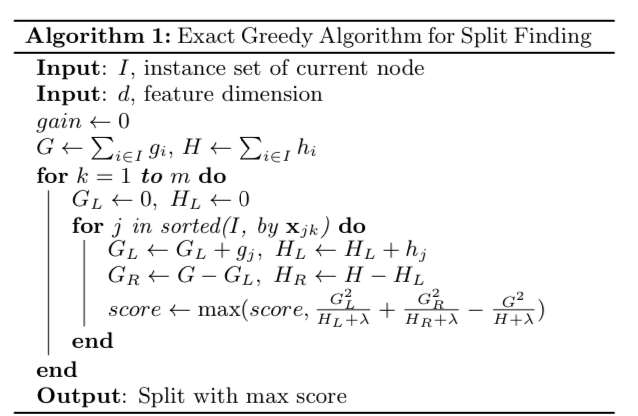
Above is the pseudocode for the exact algorithm. As demonstrated in the code, for each feature (i. e. column), the instances are sorted according to its feature value, and all the possible splits are evaluated for the loss reduction.
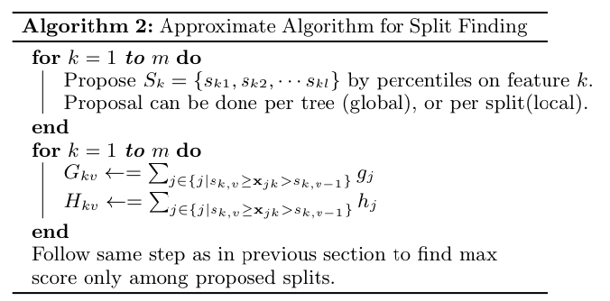
As opposed to algorithm 1, which considers all possible splits, the approximate algorithm computes the candidate split points from which the actual spliting criterion is selected. The algorithm evaluates only the splits that are contained in the candidate set $S_k$ for each feature $k$. In computing the candidate set, the authors engage in the quantile strategy where the quantile values of each feature are used as the split candidates. To elaborate, there are two variants of the approximate algorithm:
- The global variant uses the same split candidates throughout the entire trees.
- The local variant re-computes the split candidates in a per-tree basis.
Weighted Quantile Sketch
For an approximate algorithm to work, it must be provided with the split candidates for each feature. As previously mentioned, the candidates are computed as the quantile values of a specific feature. Therefore, the problem of calculating the split candidates looks if it can be reduced to the quantile sketch problem, which is a well-known problem with theoretical guarantee.
However, the problem is slightly different in that it has to calculate the weighted quantiles, where $h_i$'s serve as the weights. This is because the minimum value of the loss function,
$$\tilde{\mathcal{L}}^{(t)}(q)=-\frac{1}{2}\sum\limits_{i=1}^T\frac{\sum_{i\in I_{j}}g_i^2}{\sum_{i \in I_j} h_i+\lambda}$$
can be re-written as
$$\sum_{i=1}^n \frac{1}{2} h_i\left(f_t\left(\mathbf{x}_i\right)-g_i / h_i\right)^2+\Omega\left(f_t\right)+\text{const.},$$
which exactly is the weighted sum of squared errors. Therefore, the authors define a rank function
$$r_k(z)=\frac{1}{\sum_{(x, h) \in \mathcal{D}_k} h} \sum_{(x, h) \in \mathcal{D}_k, x<z} h$$
where $D_k={(x_{1k}, h_1), \cdots, (x_{nk}, h_n)}$ is the set of pairs of $k$-th feature values and second-order gradients. This represents the proportion of data with its $k$-th feature value less than $z$, weighted by the second-order gradient. The rank function $r_k$ is where the quantile sketch is held on, namely, weighted quantile sketch. The authors devise a novel algorithm for solving the problem, which the authors left in the appendix.
Sparsity-aware Split Finding
Finally, the authors suggest the way to handle sparse data. To make the model to be sparsity-aware, the authors added a behavior dubbed the default direction.
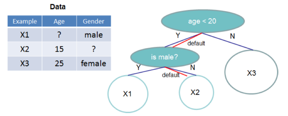
As in the figure above, the data is classified to the default direction if the feature value is missing. The default directions are learned from the data in the following modified algorithm.
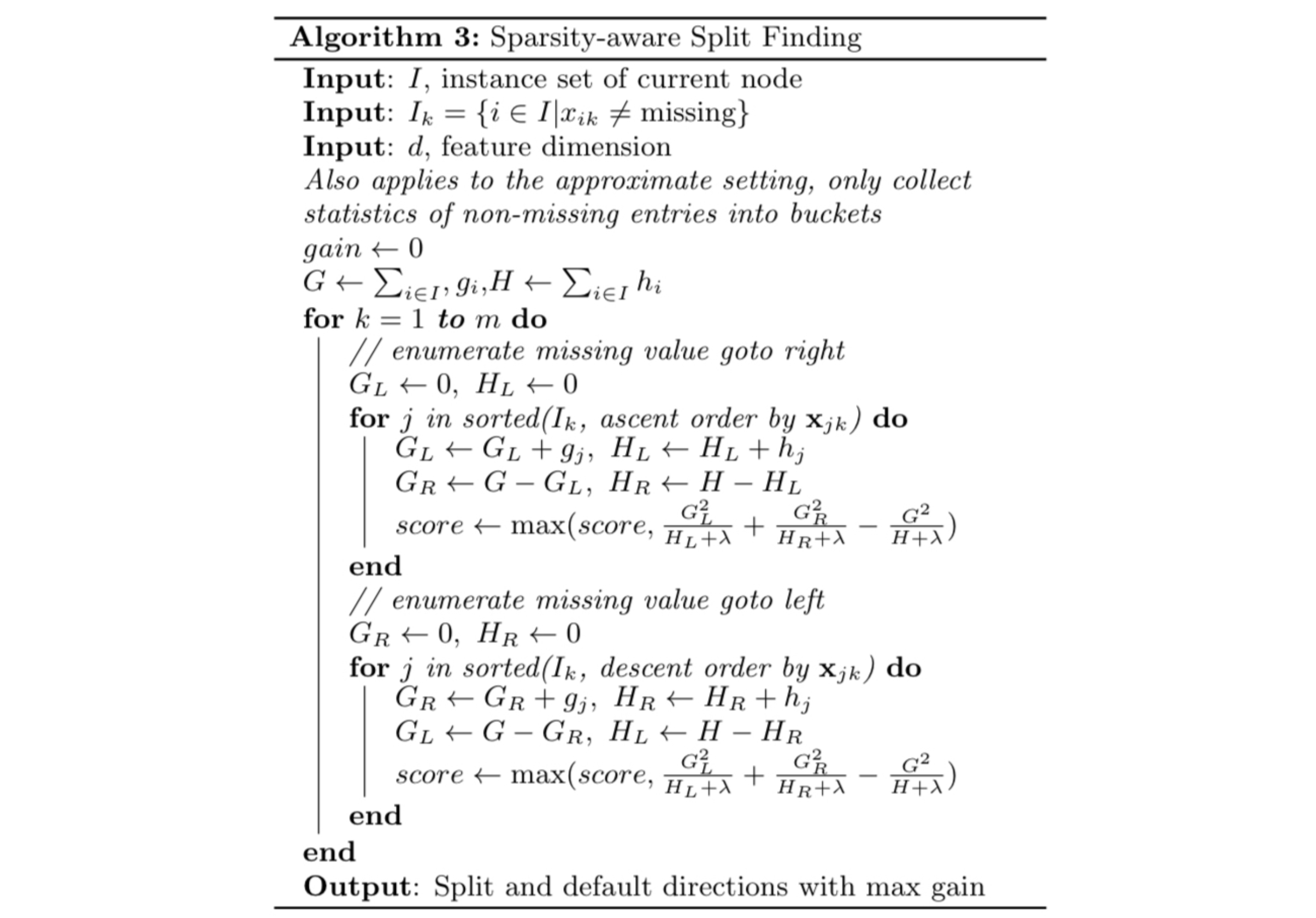
The algorithm takes both cases — where the default direction is headed left or headed right — into account, and follows the identical procedure as described above to calculate the optimal split.
By having the model be sparsity-aware, the compute complexity reduces to be linearly proportional to the number of non-zero entries in the input. For sparse datasets such as Allstate-10K, this reduces the run time more than by a factor of 50.
System Design
Column Block for Parallel Learning
The biggest overhead in the learning process is to sort the feature values. This is why the authors propose the unit of in-memory data, called the blocks. The data in each block is stored in the compressed column(CSC) format, where each column (i.e. feature) values are sorted in order, where the pointer to the corresponding gradient statistics is jointly stored.

The block structure simplifies the quantile finding procedure in the approximate algorithm into a linear scan. This is especially helpful in the case of local variant, in which quantile sketch occurs more frequently. The procedure can be parallelized to make the algorithm even faster.
The exact greedy algorithm utilizes only a single block, whereas the approximate algorithm uses multiple blocks to store the data. The blocks can be distributed across machines, or stored on disk in the case of out-of-core setting.
Cache-aware Access
Notwithstanding its reduction in time complexity, the block structure makes algorithm become cache-unfriendly. This is because the gradient statistics are accessed by their index, and therefore in a non-contiguous manner. Also, a naive implementation generates a read/write dependence in a short range.
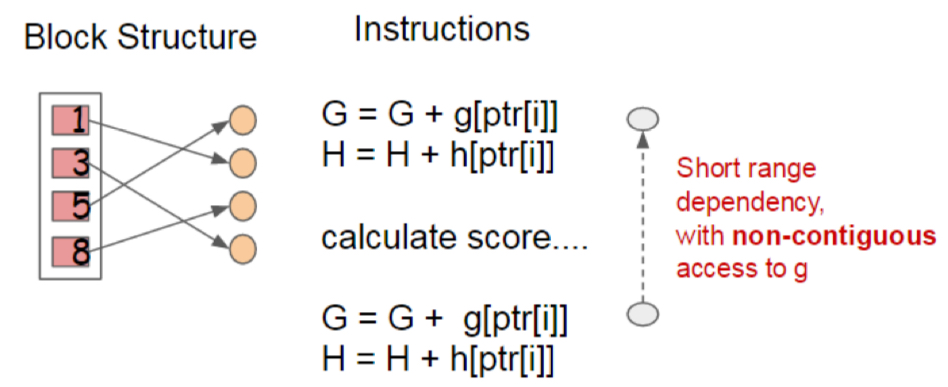
The authors ameliorate this problem by leveraging a cache-aware prefetching algorithm. To elaborate, they introduce an internal buffer in each thread where the gradient statistics are loaded in advance. Also, the authors modify the accumulation process to be held in a mini-batch manner. This elongates the distance of the depencences and reduces the memory overhead, and thereby improves the time efficienty roughly twice.

When running the approximate algorithm, choosing the appropriate block size is of great matter.
Too small block sizes lead into a overly small workload for each thread, causing an inefficienct parallelization. On the other hand, too large block sizes increases the possibility of cache miss.
A good choice of block size was selected between the two ends.
Blocks for Out-of-core Computations
To handle the data that is too large to fit into main memory, it is important to utilize the disk memory in an efficient manner. To reduce the overhead of doing so, the authors introduce two techniques for out-of-core computation:
- Block compression is a technique in which the block is saved on the disk in the compressed format, which is generated using a general-purpose compressor. The compressed on-disk data is loaded and decompressed by an independent thread on-demand.
- Block sharding is a viable option when there are multiple disks available. The method partitions the data within a single block to be stored in a number of different disks, resulting in the increase of disk reading throughput.
Code Example
XGBoost is open online to be used publicly. In this section, we will use XGBoost to solve a simple regression problem.
Import Packages
Import the packages required in our code example. Install the packages if they are unavailable.
pip install xgboost
import xgboost as xgb
import numpy as np
from sklearn import datasets
from sklearn.model_selection import train_test_split
from sklearn.metrics import mean_squared_error
from sklearn.model_selection import RandomizedSearchCV
Prepare Dataset
The dataset we are going to handle is the diabetes dataset provided by scikit-learn. The dataset can be imported using datasets.load_diabetes. Load the dataset and split them into train and test subsets.
diabetes_X, diabetes_y = datasets.load_diabetes(return_X_y=True)
X_train, X_test, y_train, y_test = train_test_split(diabetes_X, diabetes_y, test_size=0.2, random_state=42)
Define a XGBRegressor
xg_reg = xgb.XGBRegressor(objective ='reg:squarederror', colsample_bytree = 0.7, learning_rate = 0.2,
                          max_depth = 5, reg_lambda = 10, n_estimators = 100)
Define an XGBoost instance using the line above. Here are the descriptions about each argument:
objective ='reg:squarederror’ signifies that the model is fit using the regularized squared error, i.e., $l(x, y) = \lVert x-y\rVert_2^2$.colsample_bytree=0.3 specifies the subsample ratio of columns(column subsampling) when each tree is constructed. learning_rate=0.1 provides the shrinkage $\eta$ described in the paper.max_depth = 5 is the maximum depth of each tree.reg_lambda = 10 is the $L_2$ regularization coefficient. n_estimators = 100 is the number of trees used in XGBoost.
In the case of classification task, you can use xgb.XGBClassifier instead.
Hyper-parameter Search
Before we fit our model to the data, hyper-parameter search will be conducted. To do so, we will use RandomizedSearchCV module defined in scikit-learn. The module fits the given model repeatedly using randomly chosen combination of hyper-parameters, and evaluate it using cross validation (CV).
params = {'max_depth': [None, 2, 3, 5, 7, 10, 20],
          'reg_lambda': [0, 1e-3, 1e-2, 1e-1, 1, 10],
          'learning_rate': [1e-3, 3e-3, 1e-2, 3e-2, 1e-1, 3e-1],
          'n_estimators': [10, 30, 100]}

tuned_reg = RandomizedSearchCV(xg_reg, params, n_iter=20, scoring='neg_mean_squared_error', cv=5)
print(tuned_reg.get_params())
{'cv': 5, 'error_score': nan, 'estimator__objective': 'reg:squarederror', 'estimator__base_score': None, 'estimator__booster': None, 'estimator__callbacks': None, 'estimator__colsample_bylevel': None, 'estimator__colsample_bynode': None, 'estimator__colsample_bytree': 0.7, 'estimator__device': None, 'estimator__early_stopping_rounds': None, 'estimator__enable_categorical': False, 'estimator__eval_metric': None, 'estimator__feature_types': None, 'estimator__gamma': None, 'estimator__grow_policy': None, 'estimator__importance_type': None, 'estimator__interaction_constraints': None, 'estimator__learning_rate': 0.2, 'estimator__max_bin': None, 'estimator__max_cat_threshold': None, 'estimator__max_cat_to_onehot': None, 'estimator__max_delta_step': None, 'estimator__max_depth': 5, 'estimator__max_leaves': None, 'estimator__min_child_weight': None, 'estimator__missing': nan, 'estimator__monotone_constraints': None, 'estimator__multi_strategy': None, 'estimator__n_estimators': 100, 'estimator__n_jobs': None, 'estimator__num_parallel_tree': None, 'estimator__random_state': None, 'estimator__reg_alpha': None, 'estimator__reg_lambda': 10, 'estimator__sampling_method': None, 'estimator__scale_pos_weight': None, 'estimator__subsample': None, 'estimator__tree_method': None, 'estimator__validate_parameters': None, 'estimator__verbosity': None, 'estimator': XGBRegressor(base_score=None, booster=None, callbacks=None,
             colsample_bylevel=None, colsample_bynode=None,
             colsample_bytree=0.7, device=None, early_stopping_rounds=None,
             enable_categorical=False, eval_metric=None, feature_types=None,
             gamma=None, grow_policy=None, importance_type=None,
             interaction_constraints=None, learning_rate=0.2, max_bin=None,
             max_cat_threshold=None, max_cat_to_onehot=None,
             max_delta_step=None, max_depth=5, max_leaves=None,
             min_child_weight=None, missing=nan, monotone_constraints=None,
             multi_strategy=None, n_estimators=100, n_jobs=None,
             num_parallel_tree=None, random_state=None, ...), 'n_iter': 20, 'n_jobs': None, 'param_distributions': {'max_depth': [None, 2, 3, 5, 7, 10, 20], 'reg_lambda': [0, 0.001, 0.01, 0.1, 1, 10], 'learning_rate': [0.001, 0.003, 0.01, 0.03, 0.1, 0.3], 'n_estimators': [10, 30, 100]}, 'pre_dispatch': '2*n_jobs', 'random_state': None, 'refit': True, 'return_train_score': False, 'scoring': 'neg_mean_squared_error', 'verbose': 0}
Model Fitting
Finally, we fit the model using the searched hyper-parameters and evaluate the model using the test set.
tuned_reg.fit(X_train, y_train)
preds = tuned_reg.predict(X_test)
mse = mean_squared_error(y_test, preds)
print("MSE: %f" % (mse))
MSE: 2824.175276
We just solved a simple regression problem by harnessing the power of XGBoost!