Mildenhall, Ben, et al. "Nerf: Representing scenes as neural radiance fields for view synthesis." Communications of the ACM 65.1 (2021): 99-106.
NeRF is a popular paper which had pioneered a new paradigm in 3D computer vision. Today I will review NeRF and delve into the techniques that it has employed to achieve the great performance in the task of novel view synthesis.
Novel View Synthesis is a task in which a model takes several images of a single object, tagged with their respective perspectives, and predicts an image of the given object taken at a new direction. Prior approaches to tackle this task can be divided by two major classes:
- Those using discrete representations, such as triangle meshes or voxel grid,
- and more recently suggested, methods that encodes the object and the scene in the weight of an MLP
So far, first line of works have shown a more promising results. However, optimizing meshes based on the reprojected image has been a bottleneck to the mesh approach, primarily since it has a poor loss landscape and is easily attracted to local minima. Also, despite its impressive performance, the voxel grid approach lacked the ability to scale up to higher resolution because of its high time and space complexity.
For these reasons, the second line of works, introducing a multi-layer perceptron(MLP) to represent the 3D shape of the object, have been the direction of 3D computer vision in the spotlight. Popular approaches employ MLPs to approximate a function from the coordinate $(x, y, z)$ to the distance from the observer or the occupancy of that particular position. However, these methods are limited because of there requirement of ground-truth 3D geometry. More recent works have mitigated the training step to only require the 2D images, but they are also confined to rendering of simple shapes.
Introducing 5D radiance Field
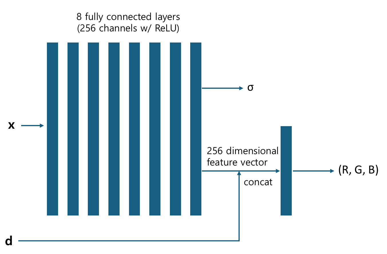
To cope with these problems, the authors suggest an approach that uses an MLP to approximate a 5D vector-valued function, which takes the viewing direction $(\theta,\phi)$ along with the position of the point $(x, y, z)$ as an input. Given these arguments, the MLP is designed to output the color $(R, G, B)$ and the volume density($\sigma$) and is dubbed the Neural Radiance Field(NeRF).
To generate a novel view using NeRF, we can follow these steps:
- Sample the 3D points from the region where the camera rays march through.
- Feed the coordinates of the sampled points and the camera direction into the NeRF, yielding the color and the volume density of each point.
- Use classical volume rendering technique to render the final 2D image from the given perspective.
Let’s dive into the details. The function can be more formally defined as follows:
$$F_{\Theta}: (\mathbf{x, d}) \to (\mathbf{c}, \sigma)$$
Here, $\mathbf{x}=(x, y, z)$ is a 3D location, $\mathbf{d} = (\theta, \phi)$ is the 2D viewing direction, $\mathbf{c}=(R, G, B)$ is an emitted color and $\sigma$ is a volume density. In practice, $\mathbf{d}$ is represented as a unit vector for that direction. The MLP uses the set of parameters $\Theta$ to represent this function.
In order to enforce the volume density $\sigma$ to be independent from the viewing direction, $F_\Theta$ first transforms the inputs with eight fully connected layers to yield 256 dimensional feature vector along with $\sigma$. After that, the direction vector $\mathbf{d}$ is concatenated to the feature vector to be fed into an additional linear layer. This additional layer outputs the color, $(R, G, B)$.

By employing this network architecture, $\sigma$ is enforced to be independent to the view direction, whereas $(R, G, B)$ takes it into account.
Volume Rendering with Radiance Fields
Now, it is time to leverage the outputs of NeRF for the rendering of the image. NeRF uses the following formula to calculate the output color of the camera ray $\mathbf{r}(t) = \mathbf{o} + t\mathbf{d}$ with near and far bound $t_n$ and $t_f$:
$$C(\mathbf{r}) = \int_{t_n}^{t_{f}}T(t) \sigma(\mathbf{r}(t))\mathbf{c}(\mathbf{r}(t), \mathbf{d})dt$$
Here, $T(t)$ is the accumulated transmittance of the ray starting at the position $t$, i. e. the probability of the light that started at the position $t$ to survive. This can be calculated interpreting $\sigma(\mathbf{r}(t))$ as the differential probability for the light ray to be terminated at the position $\mathbf{r}(t)$, thus,
$$T(t + dt) - T(t) = - T(t)\sigma(t) dt$$
Dividing the both sides by $dt$ and putting $dt\to 0$ yields:
$$\frac{dT}{dt} = -\sigma(t)T(t)\quad \Rightarrow \quad T(t) = \exp\left({-\int_{t_{n}}^{t}\sigma(\mathbf{r}(s))ds}\right)$$
Thus, the equation for $C(\mathbf{r})$ can be interpreted as the weighted sum of the lights from all the particles on the ray trajectory with weight $\sigma$, taking into account that they can be partially occluded by other particles by probability of $T(t)$. Since it is impractical to calculate the integral, its value is estimated by stratified sampling: the interval $[t_{n}, t_f]$ is evenly partitioned into $N$ pieces, from which each sample $t_i$ is uniformly sampled. These samples are exploited to calculated the estimated color $\hat{C}(\mathbf{r})$ as follows:
$$\hat{C}(\mathbf{r}) = \sum_{i=1}^{N}T_{i}(1 - \exp(-\sigma_{i}\delta_i))\mathbf{c}_{i}, \quad \text{where } T_{i}= \exp\left(-\sum_{j=1}^{i-1}\sigma_j\delta_j\right)$$
where $\delta_i=t_{i+1}-t_i$. The authors note that the equation matches with the formula for alpha compositing, where $\alpha_{i}= 1-\exp(\sigma_{i}\delta_i)$.
Optimizations: Positional Encoding and Hierarchical Sampling
Now, all the necessary components of NeRF are explained. However, the authors have introduced two optimization techniques to further improve the model’s performance. Let’s take a look at each.
Positional Encoding
NeRF introduces the positional encoding identical to that used in Transformers:
$$\gamma(p)=(\sin(2^{0}\pi p), cos(2^{0}\pi p),\cdots,\sin(2^{L-1}\pi p), cos(2^{L-1}\pi p)$$
This is adopted to augment the ability of MLP to represent high frequency functions. Since neural networks are biased to learn low frequency functions, feeding $\gamma(\mathbf{x})$ and $\gamma(\mathbf{d})$, instead of $\mathbf{x}$ and $\mathbf{d}$ respectively, can enhance the performance of the model when modeling an object with complex geometry.
Hierarchical Volume Sampling
As explained above, NeRF estimates the integral in the equation of $C(\mathbf{r})$ by sampling points from uniformly partitioned intervals. However, this strategy may be inefficient since the components that barely contribute to the light ray, such as free space of occluded region, may be oversampled. Therefore, coarse network is introduced to unequally sample points proportionately to its estimated effect on the result.
To do so, the authors reformulate the $\hat{C}(\mathbf{r})$ as the weighted sum of colors $c_i$:
$$\hat{C}_c(r)= \sum\limits_{i=1}^{N_{c}}w_ic_{i}\quad\text{where } w_{i}= T_{i}(1-\exp(-\sigma\delta_i))$$
Normalizing the weights so that $\sum\limits_i\hat{w}_i$ becomes 1 allows $\hat{w}_i$ to serve as a piecewise constant probability density function, where its value is $\hat{w}_i$ for $[t_{i}, t_{i+1}]$. Now, the fine network utilizes this PDF to sample the points needed to evaluate the integral for $\hat{C}_f(\mathbf{r})$, where both the points from the coarse network and the re-sampled points are jointly exploited to estimate the integral.
Implementation Details
One may have a misconception that NeRF is a single network trained to take a number of images as input and outputs the 3D volume rendered object. This is not how NeRF works. The neural networks are trained separately scene-specifically, and cannot be re-used for other scenes.
Considering this feature of NeRF, the authors utilized the dataset that comprises the RGB image of the scene and their corresponding camera poses. To train the NeRF for each scene, the rays are randomly selected and followed the hierarchical sampling process described in the previous section, sampling $N_c$ points from the coarse network and $N_f$ from the fine network to estimate the color $C(\mathbf{r})$. The loss function defined simply as
$$\mathcal{L} = \sum\limits_{r\in\mathcal{R}} \left[\lVert \hat{C}_c(\mathbf{r}) -C(\mathbf{r})\rVert^{2_{2}} + \lVert\hat{C}_f(\mathbf{r}) -C(\mathbf{r})\rVert^2\right]$$
The networks were trained using Adam optimizer($\beta_{1}=0.9,\beta_2=0.99$) with $\epsilon=10^{-7}$, taking approximately 1–2 days with NVIDIA V100.
Results

The paper evaluates NeRF along with the three best performing models, Scene Representation Networks(SRN), Neural Volume(NV), and Local Light Field Fusion(LLFF). As in the above table, NeRF outperformed the existing state-of-the-art models by a huge margin in the vast majority of the metrics.
The authors strongly recommend the readers to watch the video to better experience the performance of NeRF qualitatively.
Ablation Study
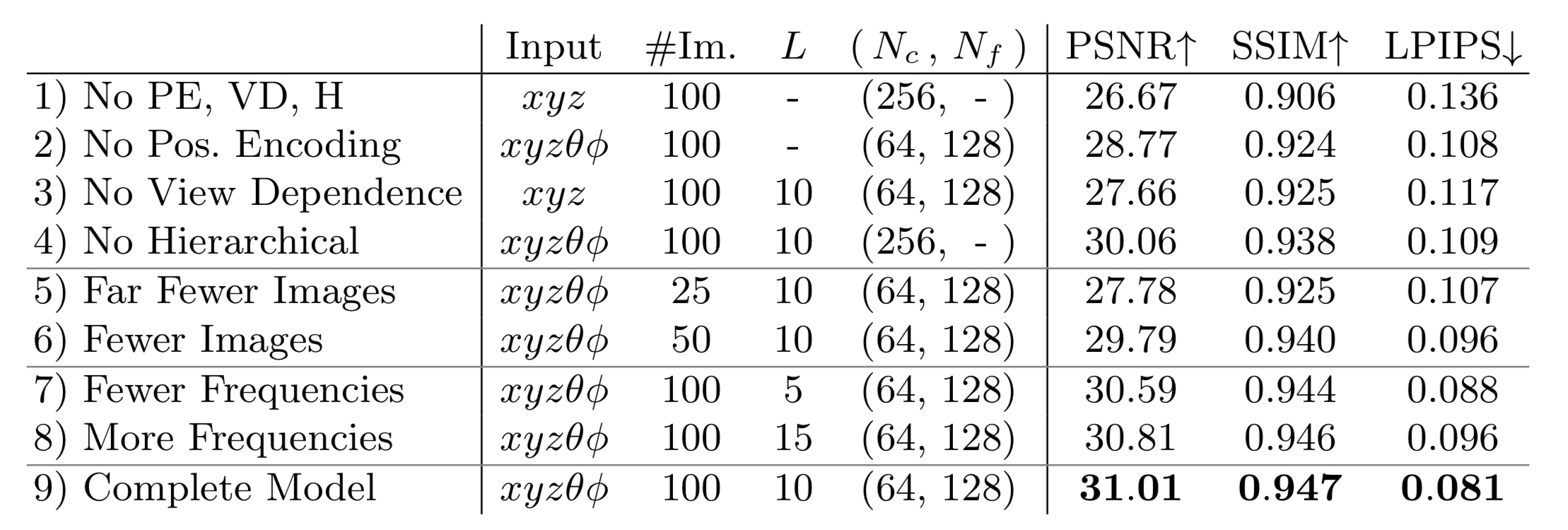
An ablation study was conducted to evaluate each of the optimizations employed in the paper: Positional Encoding(PE), View Dependence(VD) and Hierarchical Sampling(H).

As in the table above, omitting a single optimization resulted in a significant performance drop. This demonstrates that none of the optimizations were redundant. Also, the results indicate that reducing the number of images also deteriorates the performance, and introducing fewer or more frequencies in the positional embedding would be ineffective.