
[TOC]
Song, Yang, et al. "Consistency Models." International Conference on Machine Learning. PMLR, 2023.
Proposed by Yang Song et al., consistency models are a new class of generative model designed to mitigate high compute demand of existing diffusion models, circumbenting its iterative sampling. Let's dive into the key principles and mathematical foundations of consistency models.
From Diffusion Model to Probability Flow(PF) ODE
The authors emphasize that consistency models are deeply inspired from diffusion models, which is the most successful branch of generative models, achieving state-of-the-art performance across a wide range of fields. For those who are not familiar with diffusion models, I recommend you to read one of many blog posts describing diffusion models or refer to papers such as DDPM.
The forward diffusion process of DMs can be expressed as the following SDE(stochastic differential equation):
$$d\mathbf{x}_t = \mathbf{\mu}(\mathbf{x}_t, t) dt + \sigma(t) d\mathbf{w}_t, \quad t \in [0, T],$$
starting from the data distribution $p_{\text{data}}(x)$. Here, $\mathbf{w}_t$ denotes standard Brownian motion.
The authors emphasize that the above equation can be converted to a Probability Flow(PF) ODE:
$$d\mathbf{x}_t = \left[\mathbf{\mu}(\mathbf{x}_t, t) - \frac{1}{2} \sigma(t)^2 \nabla \log p_t(\mathbf{x}_t) \right]dt$$
Here, $\log\nabla p_t(\mathbf{x})$ is called the score function of $p_t(\mathbf{x})$. Note that the above equation is solved in reverse-time direction, yielding the solution at $t < T$ starting from the initial condition $x_T \sim \pi(\mathbf{x})$. Here, we assume that $\mathbf{\mu}(\mathbf{x}, t) = 0, \sigma(t) = \sqrt{2t}$ and therefore $\pi(\mathbf{x}) = \mathcal{N}(0, T^2\mathbf{I})$. As a result, $p_t(\mathbf{x}) = p_\text{data}(\mathbf{x}) \otimes \mathcal{N}(0, T^2\mathbf{I})$ where $\otimes$ denotes convolution.
However, in the above formula, computing $\nabla \log p_t(\mathbf{x})$ is actually intractible. Therefore, a score model $\mathbf{s}_\phi(\mathbf{x}, t)$ can be introduced to approximate the term (score matching). This simplifies the equation as follows:
$$\frac{d\mathbf{x}_t}{dt} = -t\mathbf{s}_\phi(\mathbf{x}_t, t).$$
Now, the sampling from the diffusion model can be done by:
- Sampling $\hat{\mathbf{x}_T} \sim \pi = \mathcal{N}(0, T^2\mathbf{I})$ as an initial condition, and then
- Solve it backwards using numerical methods, and thereby obtaining the trajectory.
The resultant $\hat{\mathbf{x}_0}$ can be seen as an approximate sample from the data distribution $p_\text{data}$.
High Computional Overhead of Diffusion Models
During inference time, one of the defining characteristics of diffusion model is the iterative process of refining noisy image into a less noisy one. This progressively generates a clear, new image from a completely random noise. However, this iterative procedure demands a lot of compute budget, since denoising steps have to be applied repeatedly to sample a new image. Also, the sequential nature of this sampling process makes the parallelization hard, causing a relatively slow inference speed.
On the other hand, the advantage of this iterative method is that it provides a trade-off so that one can choose between the image quality and the efficiency (i.e. less compute budget), simply by adjusting the number of denoising steps.
Consistency Models
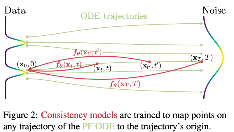
The authors aim to tackle the cost issue that stems from the iterative nature of diffusion models' sampling process, while preserving its advantage of quality-efficiency trade-off. As a result, they came up with a novel type of model that generates a new sample in a single step, namely, consistency model.
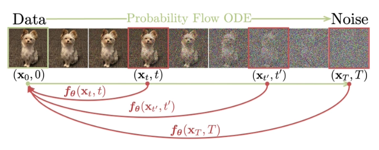
Based on the perspective that views diffusion models as a process of solving probability flow(PF) ODE, the authors defines a function that maps each point of the ODE trajectory to its starting point. Let's take a look at the authors' definition.
Definition. consistency function.
Given a solution trajectory ${\mathbf{x}_t}_{t\in[\epsilon, T]}$ of the PF ODE
$$d\mathbf{x}_t = \left[\mathbf{\mu}(\mathbf{x}_t, t) - \frac{1}{2} \sigma(t)^2 \nabla \log p_t(\mathbf{x}_t) \right]dt,$$
consistency function $\mathbf{f}: (\mathbf{x}_t, t)\mapsto \mathbf{x}_\epsilon$ is a function that satisfies self-consistency. That is, its output for an arbitrary pair $(\mathbf{x}_t, t)$ on the same PF ODE trajectory are consistent.
Parametrization
You may observe from the above definition that $\mathbf{f}(\mathbf{x}_\epsilon, \epsilon) = \mathbf{x}_\epsilon$ for any $\mathbf{x}_\epsilon$. Thus, $\mathbf{f}(\cdot, \epsilon)$ has to be an identify function. The authors decide to parametrize consistency model as follows, in order to enforce this "boundary condition":
$$\mathbf{f_\theta}(\mathbf{x}, t) = c_\text{skip}(t) \mathbf{x} + c_\text{out}(t) \mathbf{F_\theta}(\mathbf{x}, t)$$
where $c_\text{skip}(t)$ and $c_\text{out}(t)$ are differentiable functions that satisfy $c_\text{skip}(\epsilon) = 1, c_\text{out}(\epsilon) = 0$.
Sampling
Now, we have everything needed to generate a new data. Given a well-trained consistency model, the process of sampling a new data from data distribution can be summarized by the following pseudocode.
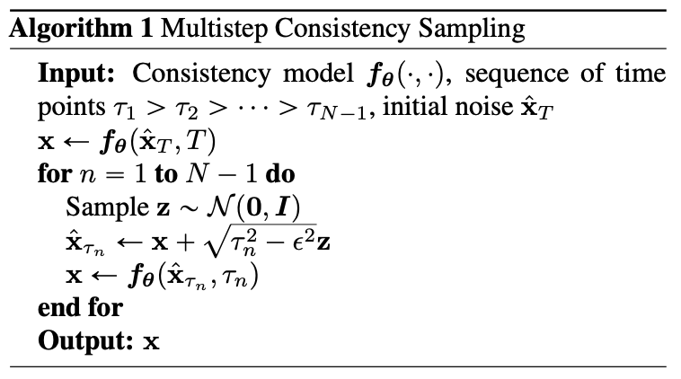
Akin to score-based diffusion models, the algorithm first samples $\hat{\mathbf{x}_T}\sim \mathcal{N}(0, T^2I)$ and solves the PF ODE in the reverse-time direction. However, it utilizes consistency function $\mathbf{f_\theta}$ as opposed to score function $\mathbf{s_\theta}$ of diffusion models. Although, the initial noise $\hat{\mathbf{x}_T}$ can be completely denoised in a single step by $\mathbf{f_\theta}(\mathbf{x}_T, T)$ theoretically, this multistep algorithm, not only enhances the quality of resultant sample but also provides flexibility to trade compute for sample quality.
Training Consistency Models via Distillation
Then how do we train a consistency model? The authors first suggest a method to train a consistency model via distillation of a pre-trained score model $\mathbf{s_\phi}(\mathbf{x}, t)$.
Assuming that the time horizon is discretized into $N-1$ subintervals, namely $t_1 = \epsilon < t_2 < \cdots < t_N = T$. By solving the PF ODE via ODE solver (in a reverse-time direction), one can obtain the estimate of sample at $t_n$ from that at $t_{n+1}$. Below is an example with Euler solver.
$$\hat{\mathbf{x}}_{t_n}^\phi = \mathbf{x}_{t_{n+1}} - (t_n - t_{n+1})t_{n+1}s_\phi(\mathbf{x}_{t_{n+1}}, t_{n+1})$$
Based on the formula, the authors could devise a distillation method using a given dataset. Given a data point $\mathbf{x}$, they could sample $\mathbf{x}_{t+1}\sim \mathcal{N}(\mathbf{x}, t_{n+1}^2\mathbf{I})$ and generate a pair of adjacent data points $(\hat{\mathbf{x}}_{t_n}^\phi, \mathbf{x}_{t_{n+1}})$. From a set of these pairs, training is held to optimize the consistency distillation loss:
$$\mathcal{L}_{CD}^N (\mathbf{\theta}, \mathbf{\theta}^-;\phi):=\mathbb{E}_{\mathbf{x}\sim p_\text{data}, n \sim \mathcal{U}[1, N-1]}[\lambda(t_n)d(\mathbf{f_\theta}(\mathbf{x}_{t_{n+1}}, t_{n+1}), \mathbf{f_{\theta^-}}(\hat{\mathbf{x}}_{t_n}^\phi, t_n))]$$
Note that $\lambda(\cdot)\in \mathbb{R}^+$ is a positive weighing function, $\mathbf{x}_{t_{n+1}}\sim \mathcal{N}(\mathbf{x};t^2_{n+1}\mathbf{I})$. Also, $\mathbf{\theta^-}$ denotes a running average of past values of $\mathbf{\theta}$ and $d$ is a metric function. The authors reports that making use of a network with parameters $\mathbf{\theta}^-$, which is referred to as "target network," greatly stabilizes the training process. They also provide theoretical justification for the consistency loss, which is omitted in this article.
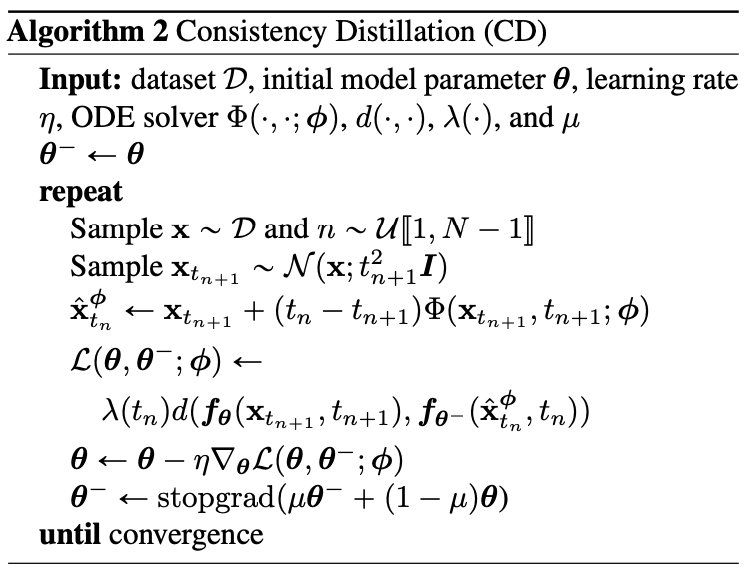
Algorithm 2 in the above figure is a distillation algorithm that is constructed based on the discussed consistency distillation loss.
Trainining Consistency Models in Isolation
The authors also propose a training method that does not rely on pre-trained score model $\mathbf{s_\phi(\mathbf{x}, t)}$. To achieve this, alternative method is required to estimate the ground truth score function $\nabla \log p_t(\mathbf{x})$. Authors demonstrate that the equation
$$\nabla \log p_t(\mathbf{x}_t) = -\mathbb{E}\left[ \frac{\mathbf{x}_t - \mathbf{x}}{t^2} | \mathbf{x}_t\right]$$
holds, where $\mathbf{x}\sim p_\text{data}, \mathbf{x}_t \sim \mathcal{N}(\mathbf{x};t^2\mathbf{I})$. This allows the estimation of the score function using a given pair of $(\mathbf{x}, \mathbf{x}_t)$. By replacing the score model, we yield the following consistency training loss, in which the proof is omitted here.
$$\mathcal{L}_{CT}^N(\theta, \theta^-)=\mathbb{E}[\lambda(t_n)d(\mathbf{f_\theta}(\mathbf{x}+t_{n+1}\mathbf{z}), \mathbf{f_{\theta^-}}(\mathbf{x}+t_n\mathbf{z}, t_n))]$$
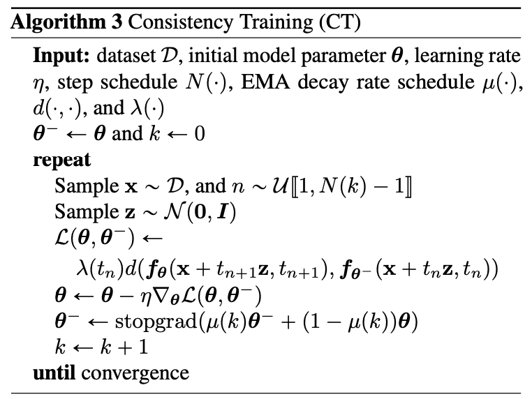
The figure above demonstrates the process of training a consistency model in isolation.